Measuring conditional correlation between financial markets' inefficiency

Fabrizio Di Sciorio; Raffaele Mattera; Juan Evangelista Trinidad Segovia; Fabrizio Di Sciorio; Raffaele Mattera; Juan Evangelista Trinidad Segovia

doi:10.3934/QFE.2023025

Quantitative Finance and Economics

2023, Volume 7, Issue 3: 491-507. doi: 10.3934/QFE.2023025

Previous Article Next Article

Research article

Measuring conditional correlation between financial markets' inefficiency

Fabrizio Di Sciorio ¹,
Raffaele Mattera ²,
Juan Evangelista Trinidad Segovia ^{1
,
,}

1.
Department of Business and Economics, University of Almeria, Spain
2.
Department of Social and Economic Sciences, Sapienza University of Rome, Italy

Received: 05 June 2023 Revised: 21 August 2023 Accepted: 21 September 2023 Published: 27 September 2023
JEL Codes: G15, G170, C58

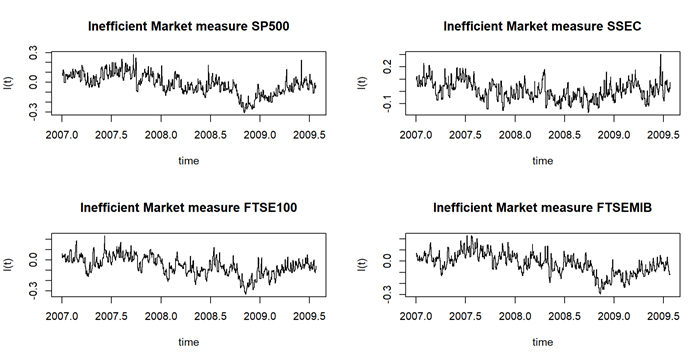
Assuming that stock prices follow a multi-fractional Brownian motion, we estimated a time-varying Hurst exponent ($ h_t $). The Hurst value can be considered a relative volatility measure and has been recently used to estimate market inefficiency. Therefore, the Hurst exponent offers a level of comparison between theoretical and empirical market efficiency. Starting from this point of view, we adopted a multivariate conditional heteroskedastic approach for modeling inefficiency dynamics in various financial markets during the 2007 financial crisis, the COVID-19 pandemic and the Russo-Ukranian war. To empirically validate the analysis, we compared different stock markets in terms of conditional and unconditional correlations of dynamic inefficiency and investigated the predicted power of inefficiency measures through the Granger causality test.
- Hurst exponent,
- efficient market hypothesis,
- dynamic conditional correlation,
- multivariate GARCH,
- Hurst-based GARCH
Citation: Fabrizio Di Sciorio, Raffaele Mattera, Juan Evangelista Trinidad Segovia. Measuring conditional correlation between financial markets' inefficiency[J]. Quantitative Finance and Economics, 2023, 7(3): 491-507. doi: 10.3934/QFE.2023025

Related Papers:

Abstract

Assuming that stock prices follow a multi-fractional Brownian motion, we estimated a time-varying Hurst exponent ($ h_t $). The Hurst value can be considered a relative volatility measure and has been recently used to estimate market inefficiency. Therefore, the Hurst exponent offers a level of comparison between theoretical and empirical market efficiency. Starting from this point of view, we adopted a multivariate conditional heteroskedastic approach for modeling inefficiency dynamics in various financial markets during the 2007 financial crisis, the COVID-19 pandemic and the Russo-Ukranian war. To empirically validate the analysis, we compared different stock markets in terms of conditional and unconditional correlations of dynamic inefficiency and investigated the predicted power of inefficiency measures through the Granger causality test.

References

[1]	Bianchi S (2005) Pathwise identification of the memory function of multifractional brownian motion with application to finance. Int J theor appl Finan 8: 255–281. https://doi.org/10.1142/S0219024905002937 doi: 10.1142/S0219024905002937
[2]	Bianchi S, Pantanella A, Pianese A (2013) Modeling stock prices by multifractional brownian motion: an improved estimation of the pointwise regularity. Quant Financ 13: 1317–1330. https://doi.org/10.1080/14697688.2011.594080 doi: 10.1080/14697688.2011.594080
[3]	Bianchi S, Pianese A (2007) Modelling stock price movements: multifractality or multifractionality? Quant Financ 7: 301–319. https://doi.org/10.1080/14697680600989618 doi: 10.1080/14697680600989618
[4]	Bianchi S, Pianese A (2018) Time-varying hurst–hoelder exponents and the dynamics of (in)efficiency in stock markets. Chaos, Soliton Fract 109: 64–75. https://doi.org/10.1016/j.chaos.2018.02.015 doi: 10.1016/j.chaos.2018.02.015
[5]	Bollerslev T (1990) Modelling the coherence in short-run nominal exchange rates: a multivariate generalized arch model. Rev Econ Stat, 498–505. https://doi.org/10.2307/2109358 doi: 10.2307/2109358
[6]	Boungou WYA (2022) The impact of the ukraine–russia war on world stock market returns. Econ Lett 215: 110516. https://doi.org/10.1016/j.econlet.2022.110516 doi: 10.1016/j.econlet.2022.110516
[7]	Cerqueti R, Mattera R (2023) Fuzzy clustering of time series with time-varying memory. Int J Approx Reason 153: 193–218. https://doi.org/10.1016/j.ijar.2022.11.021 doi: 10.1016/j.ijar.2022.11.021
[8]	Choudhry T, Jayasekera R (2014) Market efficiency during the global financial crisis: Empirical evidence from european banks. J Int Money Financ 49: 299–318. https://doi.org/10.1016/j.jimonfin.2014.03.008 doi: 10.1016/j.jimonfin.2014.03.008
[9]	Chu XWC, Qiu J (2016) A nonlinear granger causality test between stock returns and investor sentiment for chinese stock market: a wavelet-based approach. Appl Econ 48: 1915–1924. https://doi.org/10.1080/00036846.2015.1109048 doi: 10.1080/00036846.2015.1109048
[10]	Cont R (2001) Empirical properties of asset returns: stylized facts and statistical issues. Quant Financ 1: 223. https://doi.org/10.1080/713665670 doi: 10.1080/713665670
[11]	Couillard M, Davison M (2005) A comment on measuring the hurst exponent of financial time series. Physica A 348: 404–418. https://doi.org/10.1016/j.physa.2004.09.035 doi: 10.1016/j.physa.2004.09.035
[12]	Di Matteo T, Aste T, Dacorogna MM (2005) Long-term memories of developed and emerging markets: Using the scaling analysis to characterize their stage of development. J Bank Financ 29: 827–851. https://doi.org/10.1016/j.jbankfin.2004.08.004 doi: 10.1016/j.jbankfin.2004.08.004
[13]	Di Sciorio F (2020) Option pricing under multifractional brownian motion in a risk neutral framework. Stud Appl Econ 38. https://doi.org/10.25115/eea.v38i3.2902 doi: 10.25115/eea.v38i3.2902
[14]	Durcheva M, Tsankov P (2021) Granger causality networks of S & P 500 stocks. AIP Conf Proc 2333: 110014. https://doi.org/10.1063/5.0041747 doi: 10.1063/5.0041747
[15]	Engle R (2002) Dynamic conditional correlation: A simple class of multivariate generalized autoregressive conditional heteroskedasticity models. J Bus Econ Stat 20: 339–350. https://doi.org/10.1198/073500102288618487 doi: 10.1198/073500102288618487
[16]	Cannon MJ, Percival DB, Caccia DC, et al. (1997) Evaluating scaled windowed variance methods for estimating the hurst coefficient of time series. Physica A 241: 606–626. https://doi.org/10.1016/S0378-4371(97)00252-5 doi: 10.1016/S0378-4371(97)00252-5
[17]	Fernandez-Martinez M, Sanchez-Granero M, Segovia JT (2013) Measuring the self-similarity exponent in levy stable processes of financial time series. Physica A 392: 5330–5345. https://doi.org/10.1016/j.physa.2013.06.026 doi: 10.1016/j.physa.2013.06.026
[18]	Gómez-Águila A, Trinidad-Segovia J, Sánchez-Granero M (2022) Improvement in hurst exponent estimation and its application to financial markets. Financial Innovation 8: 1–21. https://doi.org/10.1186/s40854-022-00394-x doi: 10.1186/s40854-022-00394-x
[19]	Granero MS, Segovia JT, Pérez JG (2008) Some comments on hurst exponent and the long memory processes on capital markets. Physica A 387: 5543–5551.
[20]	Gripenberg G, Norros I (1996) On the prediction of fractional brownian motion. J Appl Prob 33: 400–410. https://doi.org/10.1017/S0021900200099812 doi: 10.1017/S0021900200099812
[21]	Hyndman RJ, Khandakar Y (2008) Automatic time series forecasting: the forecast package for r. J Stat Softw 27: 1–22. https://doi.org/10.18637/jss.v027.i03 doi: 10.18637/jss.v027.i03
[22]	Ito M, Noda A, Wada T (2014) International stock market efficiency: a non-bayesian time-varying model approach. Appl Econ 46: 2744–2754. https://doi.org/10.1080/00036846.2014.909579 doi: 10.1080/00036846.2014.909579
[23]	Ito M, Noda A, Wada T (2016) The evolution of stock market efficiency in the us: a non-bayesian time-varying model approach. Appl Econ 48: 621–635. https://doi.org/10.1080/00036846.2015.1083532 doi: 10.1080/00036846.2015.1083532
[24]	Kristoufek L, Vosvrda M (2013) Measuring capital market efficiency: Global and local correlations structure. Physica A 392(1):184–193. https://doi.org/10.1016/j.physa.2012.08.003 doi: 10.1016/j.physa.2012.08.003
[25]	Kristoufek L, Vosvrda M (2016) Gold, currencies and market efficiency. Physica A 449: 27–34. https://doi.org/10.1016/j.physa.2015.12.075 doi: 10.1016/j.physa.2015.12.075
[26]	Kristoufek L, Vosvrda M (2019) Cryptocurrencies market efficiency ranking: Not so straightforward. Physica A 531: 120853. https://doi.org/10.1016/j.physa.2019.04.089 doi: 10.1016/j.physa.2019.04.089
[27]	Laure M, Dutang C (2015) An r package for fitting distributions. J Stat Softw 64: 1–34.
[28]	Le Tran V, Leirvik T (2019). A simple but powerful measure of market efficiency. Financ Res Lett 29: 141–151. https://doi.org/10.1016/j.frl.2019.03.004 doi: 10.1016/j.frl.2019.03.004
[29]	Lebovits J, Lévy Vehel J (2014) White noise-based stochastic calculus with respect to multifractional brownian motion. Stochastics 86: 87–124. https://doi.org/10.1080/17442508.2012.758727 doi: 10.1080/17442508.2012.758727
[30]	Lo AW (1991) Long-term memory in stock market prices. Econometrica 59: 1279–1313. https://doi.org/10.2307/2938368 doi: 10.2307/2938368
[31]	Lo AW (2004) The Adaptive Markets Hypothesis. J Portfolio Manage 30: 15–29. https://doi.org/10.3905/jpm.2004.442611 doi: 10.3905/jpm.2004.442611
[32]	Mandelbrot BB, Van Ness JW (1968) Fractional brownian motions, fractional noises and applications. SIAM Review 10: 422–437. https://doi.org/10.1137/1010093 doi: 10.1137/1010093
[33]	Mattera R, Di Sciorio F, Trinidad-Segovia JE (2022) A composite index for measuring stock market inefficiency. Complexity. https://doi.org/10.1155/2022/9838850 doi: 10.1155/2022/9838850
[34]	Mattera R, Di Sciorio F (2021) Option pricing under multifractional process and long-range dependence. Fluct Noise Lett 20: 2150008. https://doi.org/10.1142/S0219477521500085 doi: 10.1142/S0219477521500085
[35]	Mercik S, Weron K, Burnecki K, et al. (2003) Enigma of self-similarity of fractional levy stable motions. Acta Phys Pol B 34: 3773.
[36]	Mishra PK, Das KB, Pradhan BB (2009) Empirical evidence on Indian stock market efficiency in context of the global financial crisis. Global J Financ Manage 1: 149–157.
[37]	Noda A (2016) A test of the adaptive market hypothesis using a time-varying ar model in japan. Financ Res Lett 17: 66–71. https://doi.org/10.1016/j.frl.2016.01.004 doi: 10.1016/j.frl.2016.01.004
[38]	Okorie DI, Lin B (2021) Adaptive market hypothesis: the story of the stock markets and covid-19 pandemic. N Am J Econ Financ 57. https://doi.org/10.1016/j.najef.2021.101397 doi: 10.1016/j.najef.2021.101397
[39]	Péltier RF, Lévy Véhel J (1995) Multifractional brownian motion: definition and preliminary results. Technical report, RR-2645, INRIA-00074045.
[40]	Peters EE (1994) Fractal market analysis: applying chaos theory to investment and economics, volume 24. John Wiley & Sons.
[41]	Puertas AM, Clara-Rahola J, Sánchez-Granero MA, et al. (2023) A new look at financial markets efficiency from linear response theory. Financ Res Lett 51: 103455. https://doi.org/10.1016/j.frl.2022.103455 doi: 10.1016/j.frl.2022.103455
[42]	Puertas AM, Trinidad-Segovia JE, Sánchez-Granero MA, et al. (2021) Linear response theory in stock markets. Sci Rep 11: 23076. https://doi.org/10.1038/s41598-021-02263-6 doi: 10.1038/s41598-021-02263-6
[43]	Sánchez M Á, Trinidad JE, García J, et al. (2015). The effect of the underlying distribution in hurst exponent estimation. PLoS One 10: e0127824. https://doi.org/10.1371/journal.pone.0127824 doi: 10.1371/journal.pone.0127824
[44]	Sánchez-Granero M, Balladares K, Ramos-Requena J, et al. (2020) Testing the efficient market hypothesis in latin american stock markets. Physica A 540: 123082. https://doi.org/10.1016/j.physa.2019.123082 doi: 10.1016/j.physa.2019.123082
[45]	Sensoy A, Tabak BM (2015) Time-varying long term memory in the european union stock markets. Physica A 436: 147–158. https://doi.org/10.1016/j.physa.2015.05.034 doi: 10.1016/j.physa.2015.05.034
[46]	Wang JJ, Wang XY (2021) Covid-19 and financial market efficiency: Evidence from an entropy-based analysis. Financ Res Lett 42. https://doi.org/10.1016/j.frl.2020.101888 doi: 10.1016/j.frl.2020.101888
[47]	Weron A, Weron R (2000) Fractal market hypothesis and two power-laws. Chaos Soliton Fract 11: 289–296. https://doi.org/10.1016/S0960-0779(98)00295-1 doi: 10.1016/S0960-0779(98)00295-1
[48]	Yamani E (2021) Foreign exchange market efficiency and the global financial crisis: Fundamental versus technical information. Q Rev Econ Financ 79: 74–89. https://doi.org/10.1016/j.qref.2020.05.009 doi: 10.1016/j.qref.2020.05.009
[49]	Zanin L, Marra G (2012) Rolling regression versus time‐varying coefficient modelling: An empirical investigation of the okun's law in some euro area countries. Bull Econ Res 64: 91–108. https://doi.org/10.1111/j.1467-8586.2010.00376.x doi: 10.1111/j.1467-8586.2010.00376.x

Reader Comments

Your name:*

Email:*
© 2023 the Author(s), licensee AIMS Press. This is an open access article distributed under the terms of the Creative Commons Attribution License (http://creativecommons.org/licenses/by/4.0)