Passivity analysis of discrete-time genetic regulatory networks with reaction-diffusion coupling and delay-dependent stability criteria

Yongwei Yang; Yang Yu; Chunyun Xu; Chengye Zou; Yongwei Yang; Yang Yu; Chunyun Xu; Chengye Zou

doi:10.3934/era.2025136

Electronic Research Archive

2025, Volume 33, Issue 5: 3111-3134. doi: 10.3934/era.2025136

Previous Article Next Article

Research article

Passivity analysis of discrete-time genetic regulatory networks with reaction-diffusion coupling and delay-dependent stability criteria

1.
School of Mathematics and Computer Science, Tongling University, Tongling 244061, China
2.
School of Information Science and Engineering, Yanshan University, Qinhuangdao 066004, China
3.
Department of Dermatology, Maternity and Child Health Hospital of Qinhuangdao, Qinhuangdao 066000, China

Received: 22 January 2025 Revised: 03 April 2025 Accepted: 27 April 2025 Published: 21 May 2025

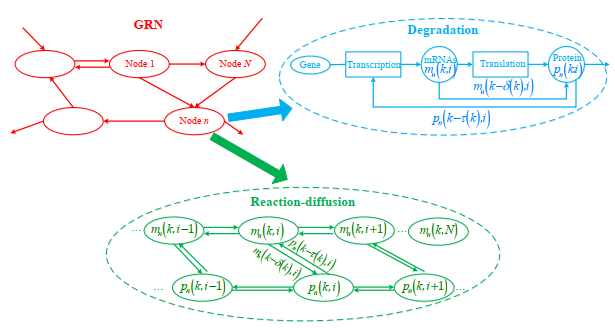
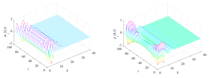
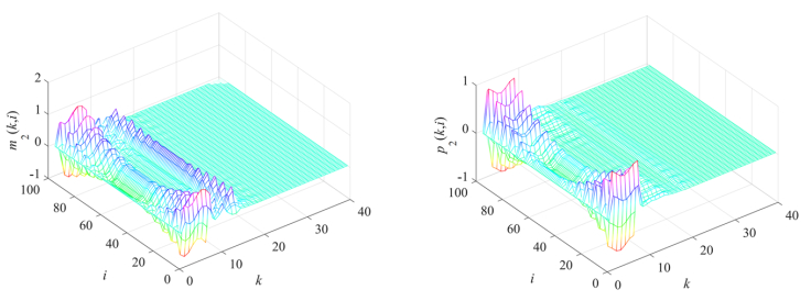
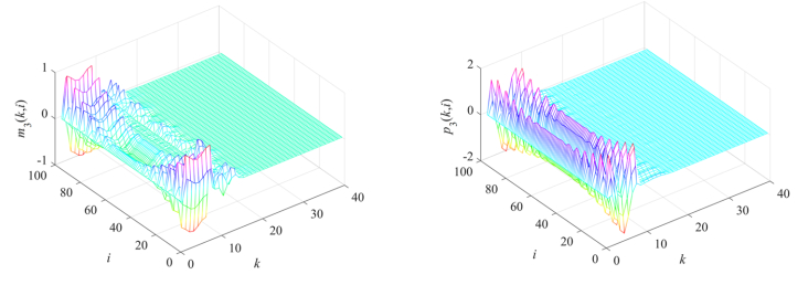
Gene regulatory networks (GRNs) play a crucial role in biological processes, with their dynamic behaviors heavily influenced by the spatial organization of genes. In particular, reaction-diffusion mechanisms govern the coupling between adjacent spatial locations in continuous time GRNs. However, traditional models often ignore the spatial coupling and reaction-diffusion properties of these networks, especially in discrete-time settings. In order to solve this problem, a new discrete-time gene regulatory network model is proposed in this paper, which explicitly considers the mutual coupling between adjacent spatial positions. To ensure the passivity of the proposed model, delay-dependent stability criteria are established by constructing appropriate Lyapunov-Krasovskii functions formulated in terms of linear matrix inequalities. To showcase the effectiveness and validity of this approach, a numerical example is presented in this paper. The results reveal that the model accurately captures the spatial coupling and reaction-diffusion nature of gene regulatory networks in discrete time settings.
- discrete-time genetic regulatory networks,
- dirichlet boundary,
- reaction-diffusion,
- linear matrix inequalities
Citation: Yongwei Yang, Yang Yu, Chunyun Xu, Chengye Zou. Passivity analysis of discrete-time genetic regulatory networks with reaction-diffusion coupling and delay-dependent stability criteria[J]. Electronic Research Archive, 2025, 33(5): 3111-3134. doi: 10.3934/era.2025136

Related Papers:

Abstract

Gene regulatory networks (GRNs) play a crucial role in biological processes, with their dynamic behaviors heavily influenced by the spatial organization of genes. In particular, reaction-diffusion mechanisms govern the coupling between adjacent spatial locations in continuous time GRNs. However, traditional models often ignore the spatial coupling and reaction-diffusion properties of these networks, especially in discrete-time settings. In order to solve this problem, a new discrete-time gene regulatory network model is proposed in this paper, which explicitly considers the mutual coupling between adjacent spatial positions. To ensure the passivity of the proposed model, delay-dependent stability criteria are established by constructing appropriate Lyapunov-Krasovskii functions formulated in terms of linear matrix inequalities. To showcase the effectiveness and validity of this approach, a numerical example is presented in this paper. The results reveal that the model accurately captures the spatial coupling and reaction-diffusion nature of gene regulatory networks in discrete time settings.

References

[1]	J. Hasty, D. McMillen, F. Isaacs, J. J. Collins, Computational studies of gene regulatory networks: in numero molecular biology, Nat. Rev. Genet., 2 (2001), 268–279. https://doi.org/10.1038/35066056 doi: 10.1038/35066056
[2]	N. Bernaola, M. Michiels, P. Larrañaga, C. Bielza, Learning massive interpretable gene regulatory networks of the human brain by merging Bayesian networks, PloS Comput. Biol., 19 (2023), 1011443. https://doi.org/10.1371/journal.pcbi.1011443 doi: 10.1371/journal.pcbi.1011443
[3]	J. Musilova, Z. Vafek, B. L. Puniya, R. Zimmer, T. Helikar, K. Sedlar, Augusta: From RNA-Seq to gene regulatory networks and Boolean models, Comput. Struct. Biotechnol. J., 23 (2024), 783–790. https://doi.org/10.1016/j.csbj.2024.01.013 doi: 10.1016/j.csbj.2024.01.013
[4]	G. Karlebach, P. N. Robinson, Computing minimal Boolean models of gene regulatory networks, J. Comput. Biol., 31 (2024), 117–127. https://doi.org/10.1089/cmb.2023.0122 doi: 10.1089/cmb.2023.0122
[5]	I. Hossai, V. Fanfani, J. Fischer, J. Quackenbush, R. Burkholz, Biologically informed NeuralODEs for genome-wide regulatory dynamics, Genome Biol., 25 (2024), 127. https://doi.org/10.1186/s13059-024-03264-0 doi: 10.1186/s13059-024-03264-0
[6]	X. She, L. Wang, Y. Zhang, Finite-time stability of genetic regulatory networks with nondifferential delays, IEEE Trans. Circuits Syst. II: Express Briefs, 70 (2023), 2107–2111. https://doi.org/10.1109/TCSII.2022.3233797 doi: 10.1109/TCSII.2022.3233797
[7]	T. Zhang, Y. Li, Exponential Euler scheme of multi-delay Caputo-Fabrizio fractional-order differential equations, Appl. Math. Lett., 124 (2022), 107709. https://doi.org/10.1016/j.aml.2021.107709 doi: 10.1016/j.aml.2021.107709
[8]	A. Polynikis, S. J. Hogan, M. D. Bernardo, Comparing different ODE modelling approaches for gene regulatory networks, J. Theor. Biol., 261 (2009), 511–530. https://doi.org/10.1016/j.jtbi.2009.07.040 doi: 10.1016/j.jtbi.2009.07.040
[9]	M. Kchaou, G. Narayanan, M. S. Ali, S. Sanober, G. Rajchakit, B. Priya, Finite-time Mittag-Leffler synchronization of delayed fractional-order discrete-time complex-valued genetic regulatory networks: Decomposition and direct approaches, Inf. Sci., 664 (2024), 120337. https://doi.org/10.1016/j.ins.2024.120337 doi: 10.1016/j.ins.2024.120337
[10]	K. Xie, C. Zhang, S. Lee, Y. Liu, C. Zhai, Sector bound-dependent matrix-separation-based inequality and its application to stability analysis of discrete-time delayed genetic regulatory networks, IEEE Trans. Circuits Syst. II: Express Briefs, 71 (2024), 3785–3789. https://doi.org/10.1109/TCSII.2024.3367777 doi: 10.1109/TCSII.2024.3367777
[11]	K. Mathiyalagan, R. Sakthivel, Robust stabilization and H_∞ control for discrete-time stochastic genetic regulatory networks with time delays, Can. J. Phys., 90 (2012), 939–953. https://doi.org/10.1139/p2012-088 doi: 10.1139/p2012-088
[12]	Q. Li, H. Q. Wei, D. Hua, J. Wang, J. Yang, Stabilization of semi-Markovian jumping uncertain complex-valued networks with time-varying delay: A sliding-mode control approach, Neural Process Lett., 56 (2024), 111. https://doi.org/10.1007/s11063-024-11585-1 doi: 10.1007/s11063-024-11585-1
[13]	G. Narayanan, M. S. Ali, H. Alsulami, T. Saeed, B. Ahmad Synchronization of T–S fuzzy fractional-order discrete-time complex-valued molecular models of mRNA and protein in regulatory mechanisms with leakage effects, Neural Process Lett., 55 (2023), 3305–3331. https://doi.org/10.1007/s11063-022-11010-5 doi: 10.1007/s11063-022-11010-5
[14]	H. Wei, K. Zhang, M. Zhang, Q. Li, J. Wang, Dissipative synchronization of Semi-Markovian jumping delayed neural networks under random deception attacks: An event-triggered impulsive control strategy, J. Franklin Inst., 361 (2024), 106835. https://doi.org/10.1016/j.jfranklin.2024.106835 doi: 10.1016/j.jfranklin.2024.106835
[15]	S. Pandiselvi, R. Raja, J. Cao, G. Rajchakit, B. Ahmad, Approximation of state variables for discrete-time stochastic genetic regulatory networks with leakage, distributed, and probabilistic measurement delays: A robust stability problem, Adv. Differ. Equations, 2018 (2018), 123. https://doi.org/10.1186/s13662-018-1569-z doi: 10.1186/s13662-018-1569-z
[16]	Y. Zhao, H. Wu, Fixed/Prescribed stability criterions of stochastic system with time-delay, AIMS Math., 9 (2024), 14425–14453. https://doi.org/10.3934/math.2024701 doi: 10.3934/math.2024701
[17]	T. Zhang, Z. Li, Switching clusters' synchronization for discrete space-time complex dynamical networks via boundary feedback controls, Pattern Recognit., 143 (2023), 109763. https://doi.org/10.1016/j.patcog.2023.109763 doi: 10.1016/j.patcog.2023.109763
[18]	R. Liang, J. Wang, PD control for passivity of coupled reaction-diffusion neural networks with multiple state couplings or spatial diffusion couplings, Neurocomputing, 489 (2022), 558–569. https://doi.org/10.1016/j.neucom.2021.12.070 doi: 10.1016/j.neucom.2021.12.070
[19]	P. U. Avila, T. Padvitski, A. C. Leote, H. Chen, J. Saez-Rodriguez, M. Kann, et al., Gene regulatory networks in disease and ageing, Nat. Rev. Nephrol., 20 (2024), 616–633. https://doi.org/10.1038/s41581-024-00849-7 doi: 10.1038/s41581-024-00849-7
[20]	P. Jothiappan, M. Kalidass, Robust passivity analysis of stochastic genetic regulatory networks with Levy noise, Int. J. Control Autom. Syst., 20 (2022), 3241–3251. https://doi.org/10.1007/s12555-021-0552-8 doi: 10.1007/s12555-021-0552-8
[21]	Y. Qin, F. Li, J. Wang, H. Shen, Extended dissipative synchronization of reaction-diffusion genetic regulatory networks based on sampled-data control, Neural Process Lett., 55 (2023), 3169–3183. https://doi.org/10.1007/s11063-022-11003-4 doi: 10.1007/s11063-022-11003-4
[22]	X. Song, X. Li, S. Song, C. K. Ahn, State observer design of coupled genetic regulatory networks with Reaction-diffusion terms via time-space sampled-data communications, IEEE/ACM Trans. Comput. Biol. Bioinf., 19 (2022), 3704–3714. https://doi.org/10.1109/TCBB.2021.3114405 doi: 10.1109/TCBB.2021.3114405
[23]	Y. Zhang, H. Liu, H. Yan, J. Zhou, Oscillatory behaviors in genetic regulatory networks mediated by microRNA with time delays and reaction-diffusion terms, IEEE Trans. Nanobiosci., 16 (2017), 166–176. https://doi.org/10.1109/TNB.2017.2675446 doi: 10.1109/TNB.2017.2675446
[24]	C. Ma, Q. Zeng, L. Zhang, Y. Zhu, Passivity and passification for Markov jump genetic regulatory networks with time-varying delays, Neurocomputing, 136 (2014), 321–326. https://doi.org/10.1016/j.neucom.2013.12.028 doi: 10.1016/j.neucom.2013.12.028
[25]	X. Zhang, Y. Han, L. Wu, Y. Wang, State estimation for delayed genetic regulatory networks with reaction-diffusion terms, IEEE Trans. Neural Networks Learn. Syst., 29 (2018), 299–309. https://doi.org/10.1109/TNNLS.2016.2618899 doi: 10.1109/TNNLS.2016.2618899

Reader Comments

Your name:*

Email:*
© 2025 the Author(s), licensee AIMS Press. This is an open access article distributed under the terms of the Creative Commons Attribution License (http://creativecommons.org/licenses/by/4.0)