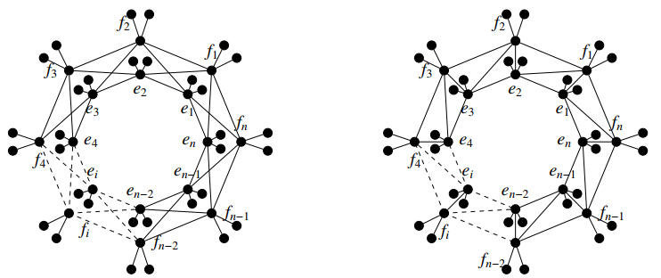
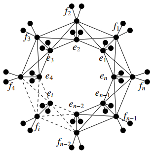
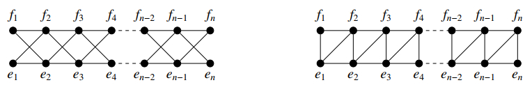
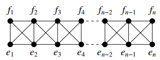
Loading [MathJax]/jax/element/mml/optable/GeneralPunctuation.js
Research article Special Issues

Algebraic invariants of edge ideals of some bristled circulant graphs

  • Let S be a polynomial ring over a field K and I be the edge ideal associated with the bristled graph of some four or five regular circulant graph. We discuss the depth, projective dimension, regularity and Stanley depth of S/I.

    Citation: Ibad Ur Rehman, Mujahid Ullah Khan Afridi, Muhammad Ishaq, Asim Asiri, Aftab Hussain. Algebraic invariants of edge ideals of some bristled circulant graphs[J]. AIMS Mathematics, 2025, 10(5): 11330-11348. doi: 10.3934/math.2025515

    Related Papers:

    [1] Bakhtawar Shaukat, Muhammad Ishaq, Ahtsham Ul Haq . Algebraic invariants of edge ideals of some circulant graphs. AIMS Mathematics, 2024, 9(1): 868-895. doi: 10.3934/math.2024044
    [2] Tazeen Ayesha, Muhammad Ishaq . Some algebraic invariants of the edge ideals of perfect $ [h, d] $-ary trees and some unicyclic graphs. AIMS Mathematics, 2023, 8(5): 10947-10977. doi: 10.3934/math.2023555
    [3] Naeem Ud Din, Muhammad Ishaq, Zunaira Sajid . Values and bounds for depth and Stanley depth of some classes of edge ideals. AIMS Mathematics, 2021, 6(8): 8544-8566. doi: 10.3934/math.2021496
    [4] Zahid Iqbal, Muhammad Ishaq . Depth and Stanley depth of edge ideals associated to some line graphs. AIMS Mathematics, 2019, 4(3): 686-698. doi: 10.3934/math.2019.3.686
    [5] Malik Muhammad Suleman Shahid, Muhammad Ishaq, Anuwat Jirawattanapanit, Khanyaluck Subkrajang . Depth and Stanley depth of the edge ideals of multi triangular snake and multi triangular ouroboros snake graphs. AIMS Mathematics, 2022, 7(9): 16449-16463. doi: 10.3934/math.2022900
    [6] Jovanny Ibarguen, Daniel S. Moran, Carlos E. Valencia, Rafael H. Villarreal . The signature of a monomial ideal. AIMS Mathematics, 2024, 9(10): 27955-27978. doi: 10.3934/math.20241357
    [7] Tariq Alraqad, Hicham Saber, Rashid Abu-Dawwas . Intersection graphs of graded ideals of graded rings. AIMS Mathematics, 2021, 6(10): 10355-10368. doi: 10.3934/math.2021600
    [8] Pradeep Singh, Sahil Sharma, Sunny Kumar Sharma, Vijay Kumar Bhat . Metric dimension and edge metric dimension of windmill graphs. AIMS Mathematics, 2021, 6(9): 9138-9153. doi: 10.3934/math.2021531
    [9] S. Masih Ayat, S. Majid Ayat, Meysam Ghahramani . The independence number of circulant triangle-free graphs. AIMS Mathematics, 2020, 5(4): 3741-3750. doi: 10.3934/math.2020242
    [10] Fida Moh'd, Mamoon Ahmed . Simple-intersection graphs of rings. AIMS Mathematics, 2023, 8(1): 1040-1054. doi: 10.3934/math.2023051
  • Let S be a polynomial ring over a field K and I be the edge ideal associated with the bristled graph of some four or five regular circulant graph. We discuss the depth, projective dimension, regularity and Stanley depth of S/I.


    Let S=K[e1,,el] be the polynomial ring over the field K, equipped with the standard grading. Let M be a finitely generated graded S-module and suppose that M has the following minimal free resolution:

    0 jZS(j)βr,j(M)jZS(j)βr1,j(M)jZS(j)β0,j(M)M 0.

    Let us denote the Castelnuovo-Mumford regularity of a module M as reg(M). Then, reg(M)=max{ji:βi,j(M)0}. The projective dimension of a module M, denoted as pdim(M), is defined as pdim(M)=max{i:βi,j(M)0}.

    Let G=(V(G),E(G)), be a graph with vertex set V(G)={e1,,el} and edge set E(G). All graphs considered in this paper are simple, finite, and undirected. The degree of a vertex is the number of edges incident on it. The edge ideal of a graph G is the squarefree monomial ideal I(G)=(eiej:{ei,ej}E(G)). If I is a monomial ideal and G(I) represents the minimal system of monomial generators of I, then supp(I):={ ei:ei|a for some aG(I)}. For mR, m:=max{bZ:bm} and m:=min{bZ:bm}. Let l2 be an integer and A be a subset of {1,,l2}. A circulant graph Cl(A) is a graph with vertex set {e1,,el} such that {ei,ej}E(Cl(A)) if and only if |ij|A or l-|ij|A. It is worth noting that Cl(A) can be considered as a generalized cycle since Cl=Cl({1}). For simplicity, the graph Cl({b1,,bm}) is denoted as Cl(b1,,bm). A circulant graph Cl(b1,,bm) is 2m regular, except in the case when 2bm=l, in which case it is (2m1) regular. Let t1, and G be a graph. Then, the graph G is called the t-fold bristled graph of G if we add t pendants to each vertex of the graph G. For a graph G, the t-fold bristled graph of G is denoted by Brt(G). There are many applications of circulant graphs in group theory [1] and network theory [2, 3].

    This paper draws inspiration from the recent work of Shaukat et al. [4], which specifically explores the algebraic invariants of the residue class rings of the edge ideals of some four and five regular circulant graphs, namely, C2n(1,n1), C2n(1,2), and C2n(1,n1,n), where n3. For n3 and t1, if Dn,t, En,t, and Fn,t represent the bristled graphs of these graphs, respectively, then Dn,t:=Brt(C2n(1,n1)), En,t:=Brt(C2n(1,2)), and Fn,t:=Brt(C2n(1,n1,n)). This study aims to investigate the regularity, depth, and Stanley depth of the residue class rings of the edge ideals of Dn,t, En,t, and Fn,t. These graphs are shown in Figures 1 and 2. Before proving our main results, we further require investigating the said algebraic invariants of the residue class rings of the edge ideals of various subgraphs of these graphs. These supporting results are obtained in Section 3. We prove our main results in Section 4. We prove the following main theorems for regularity.

    Theorem 1.1. Let n3, t1, and S=K[V(Dn,t)]. Then,

    reg(S/I(Dn,t))={n,if n is even;n1,if n is odd.

    Theorem 1.2. Let n3, t1, and S=K[V(En,t)]. Then,

    reg(S/I(En,t))={2n13,if n0,1(mod3);2n131,if n2(mod3),

    Theorem 1.3. Let n3, t1, and S=K[V(Fn,t)]. Then,

    reg(S/I(Fn,t))=n12.

    We prove the following main result for depth and Stanley depth.

    Theorem 1.4. Let n3, and S=K[V(Dn,t)]. Then,

    sdepth(S/I(Dn,t))depth(S/I(Dn,t))={n(t+1),if n is odd;n(t+1)+t1,if n is even.
    Figure 1.  From left to right Dn,2 and En,2.
    Figure 2.  Fn,2.

    We acknowledge the use of CoCoA [5] and Macaulay2 [6] during our experimental calculations. These software tools have limitations when generators of the edge ideal increases. In such scenarios, additional mathematical calculations and theoretical frameworks are necessary to compute the algebraic invariants that cannot be computed by these software packages.

    In this section, we present some definitions and findings that are extensively used in the subsequent sections of this paper. Let M be a finitely generated Zl-graded S-module. A Stanley decomposition of M is a presentation of the K-vector space M as a finite direct sum:

    T:M=zj=1ujK[Wj],

    where ujM is a homogeneous element, Wj{e1,,el}, and ujK[Wj] is a K-subspace of M generated by ujb, where b is a monomial in K[Wj]. The Zl-graded K-subspace ujK[Wj] of M is called a Stanley space of dimension |Wj| if ujK[Wj] is a free K[Wj]-module. The Stanley depth of T is defined as sdepth(T)=min{|Wj|:j=1,,z}, and the Stanley depth of M is defined as sdepth(M)=max{sdepth(T):T is a Stanley decomposition of M}. In 1982, Stanley conjectured in [7] that for a Zl-graded module M, sdepth(M)depth(M). In 2016, Duval et al. disproved this conjecture in [8] by providing a counter example. Stanley depth has gained attention, particularly when Herzog et al. presented an algorithm in [9] for computing sdepth(M) for modules of the form M=Q1/Q2, where Q2Q1S are monomial ideals. This algorithm is useful for studying Stanley depth in certain special cases. However, calculating Stanley depth using this algorithm is generally a challenging combinatorial problem. Therefore, finding Stanley depth for particular classes of modules is useful, see for instance [10, 11, 12].

    Lemma 2.1. ([13, Lemma 3.3]). Let IS be a squarefree monomial ideal such that supp(I)={e1,e2,,el}. Suppose β:=ei1ei2eirS/I and ejβI for all ej{e1,e2,,el}supp(β). Then, sdepth(S/I)r.

    The following lemmas are important for finding lower bounds for depth and Stanley depth of modules.

    Lemma 2.2 ([14]). If 0MMM is a short exact sequence of modules over a Noetherian graded ring with S_0 local, or a local ring S , then

    (a) \text{depth} (M) \geq \min\{\text{depth}(M''), \text{depth}(M')\} .

    (b) \text{depth} (M') \geq \min\{\text{depth}(M), \text{depth}(M'') + 1\} .

    (c) \text{depth} (M'') \geq \min\{\text{depth}(M')-1, \text{depth}(M)\} .

    Lemma 2.3. ([15, Lemma 2.2]). Let 0\rightarrow M' \rightarrow M \rightarrow M'' \rightarrow 0 be a short exact sequence of a {\mathbb{Z}}^{l} -graded S -module. Then, \text{sdepth}{(M)}\geq \min \{ \text{sdepth}{(M')}, \text{sdepth}{(M'')}\}.

    Lemma 2.4. ([16, Theorem 4.7]). If I is a monomial ideal and e is a variable in S , then

    (a) \text{reg} (S/I_) = 1+\text{reg} (S/(I_:e)) , if \text{reg} (S/(I_, e)) < \text{reg} (S/(I_:e)).

    (b) \text{reg} (S/I_) = \text{reg} (S/(I_, e)) if \text{reg} (S/(I_:e)) < \text{reg} (S/(I_, e)).

    (c) \text{reg} (S/I_)\in \{\text{reg} (S/(I_, e)), \text{reg} (S/(I_, e))+1\}, if \text{reg} (S/(I_:e)) = \text{reg} (S/(I_, e)).

    Lemma 2.5. ([17, Proposition 2.2.20]). Let I_1 and I_2 be monomial ideals, I_1 \subset \mathcal{S'} = K[e_{1}, \dots, e_{p}] and I_2 \subset \mathcal{S''} = K[e_{p+1}, \dots, e_{l}], where 1\leq p < l, and S = \mathcal{S'} \otimes_K \mathcal{S''}. Then, S/(I_{1}+I_{2})\cong \mathcal{S'}/I_{1} \otimes_{K}\mathcal{S''}/I_{2}.

    Lemma 2.6. ([17, Proposition 2.2.21]). Let I_1 \subset S' = K[e_1, \dotso, e_p] , I_2 \subset S'' = K[e_{p+1}, \dotso, e_{l}] be monomial ideals, where 1 \leq p < {l} . If S = S' \otimes_K S'' , then

    \text{depth}{(S'/I_1\otimes_K S''/I_2)} = \text{depth} {(S/(I_1S+I_2S)))} = \text{depth}_{S'}{(S'/I_1)}+\text{depth}_{S''}{(S''/I_2)}.

    A vertex of degree one in a graph is termed as a pendant vertex or leaf. A vertex that is not a leaf is called an internal vertex. For r \geq 2 , a star graph denoted as {S}_r is a graph with one internal vertex and r leaves connected to it. For p\geq 2 , a path on p vertices is denoted as P_p , and for p\geq 3 a cycle on p vertices is denoted as C_p . Let S_{p, t}: = Br_{t}(P_p) and C_{p, t}: = Br_{t}(C_p) .

    Lemma 2.7 ([18]). Let S = K[\mathcal{V}(S_r)] and I = I(S_{r}) . Then,

    \text{depth}(S/I) = \text{reg}(S/I) = \text{sdepth}(S/I) = 1.

    Lemma 2.8. ([19, Theorem 2.28]). Let S = K[\mathcal{V}(S_{p, t})] and I = I(S_{p, t}) . Then,

    (a) \text{reg}(S/I) = \lceil\frac{p}{2}\rceil.

    (b) \text{depth}(S/I) = \text{sdepth}(S/I) = \lceil\frac{p}{2}\rceil+\lceil\frac{p-1}{2}\rceil t.

    Lemma 2.9. ([19, Theorem 2.30 and Theorm 2.9]). Let S = K[\mathcal{V}(C_{p, t})] and I = I(C_{p, t}) . Then,

    (a) \text{reg}(S/I) = \lceil\frac{p-1}{2}\rceil.

    (b) \text{depth}(S/I) = \text{sdepth}(S/I) = \lceil\frac{p-1}{2}\rceil+\lceil\frac{p}{2}\rceil t.

    Lemma 2.10. ([15, Corollary 1.3] and [20, Proposition 2.7]). Let I\subset S be a monomial ideal. Then, for all monomials a \notin I ,

    (a) \text{depth}({S/(I:a))} \geq \text{depth}{(S/I)}.

    (b) \text{sdepth}{(S/I)} \leq \text{sdepth}{(S/(I:a))}.

    Lemma 2.11. ([21, Lemma 2.13]). Let I_{1} \subset S' = K[e_1, \dotso, e_p] , I_{2} \subset S'' = K[e_{p+1}, \dotso, e_{l}] be monomial ideals, where 1 \leq p < l and S = S' \otimes_K S'' . Then,

    \text{sdepth}{(S'/I_{1}\otimes_K S''/I_{2})} = \text{sdepth}{(S/(I_1S+I_2S))} \geq \text{sdepth}_{S'}{(S'/I_{1})} + \text{sdepth}_{S''}{(S''/I_2)}.

    Lemma 2.12. ([9, Lemma 3.6] and [22, Lemma 3.5]). Let I\subset S be a monomial ideal. If S' = S\otimes_K K[e_{{l}+1}] \cong S[e_{{l}+1}], then

    (a) \text{depth}{(S'/IS')} = \text{depth}(S/I)+1.

    (b) \text{sdepth}{(S'/IS')} = \text{sdepth}(S/I)+1.

    (c) \text{reg}{(S'/IS')} = \text{reg}(S/I).

    The following lemma is proved by Kalai et al. [23, Theorem 1.4] for squarefree monomial ideals. Herzog further extended this result to any monomial ideal [24, Corollary 3.2].

    Lemma 2.13. For monomial ideals I_{1} and I_{2} of S , \text{reg}({S/(I_{1}+I_{2})}) \leq \text{reg}(S/I_{1})+\text{reg}(S/I_{2}).

    A graph G is a weakly chordal graph if neither G nor its complement graph G^{c} contain an induced cycle of length n\geq 5. A matching, denoted by \mathcal{M} , in a graph G is a subset of \mathsf{E}(G) where there is no common vertex between any pair of edges. A matching that forms an induced subgraph of G is referred to as a induced matching in G . Furthermore, \text{indmat}(G) represents the induced matching number of graph G , which is defined as follows: \text{indmat}(G) = \max \{|\mathcal{M}|: \, \, \mathcal{M} \text{ is an induced matching in } G \}.

    Lemma 2.14. ([25, Lemma 2.2] and [26, Corollary 6.9]). For a finite simple graph G , \text{reg}(S/I(G))\geq \text{indmat}(G). Furthermore, for a chordal graph G , \text{indmat}(G) = \text{reg}(S/I(G)) .

    Lemma 2.15. ([27, Theorem 14]). For a weakly chordal graph G , \text{indmat}(G) = \text{reg}(S/I(G)) .

    Lemma 2.16. ([28, Lemma 3.2]). Let 1\leq p < l . If I_{1}\subset \mathcal{S'} = K[e_{1}, \dots, e_{p}] and I_{2}\subset \mathcal{S''} = K[e_{p+1}, \dots, e_{l}] are non-zero homogeneous ideals of \mathcal{S'} and \mathcal{S''} and we regard I_{1}+I_{2} as a homogeneous ideal of S = \mathcal{S'} \otimes_K \mathcal{S}'', then

    \text{reg}({S/(I_{1}+I_{2}})) = \text{reg}(\mathcal{S'}/I_{1})+\text{reg}(\mathcal{S''}/I_{2}).

    For n\geq 1 , let \mathbb{A}_n , \mathbb{B}_{n} , and \mathbb{C}_{n} be subgraphs of {C}_{2n}(1, n-1) , {C}_{2n}(1, 2) , and {C}_{2n}(1, n-1, n) , respectively. Subgraphs \mathbb{A}_n , \mathbb{B}_{n} , and \mathbb{C}_{n} are shown in Figures 3 and 4. Let us denote the the t -fold bristled graphs of \mathbb{A}_n , \mathbb{B}_{n} , and \mathbb{C}_{n} as follows: \mathbb{A}_{n, t}: = Br_t(\mathbb{A}_n), \mathbb{B}_{n, t}: = Br_t(\mathbb{B}_n) , and \mathbb{C}_{n, t}: = Br_t(\mathbb{C}_n).

    Figure 3.  From left to right \mathbb{A}_n and \mathbb{B}_{n}. .
    Figure 4.  \mathbb{C}_{n} .

    In this section, we compute the regularity of the cyclic modules K[\mathcal{V}(\mathbb{A}_{n, t})]/I(\mathbb{A}_{n, t}), K[\mathcal{V}(\mathbb{B}_{n, t})]/I(\mathbb{B}_{n, t}) , and K[\mathcal{V}(\mathbb{C}_{n, t})]/I(\mathbb{C}_{n, t}). We also compute depth, Stanley depth, and projective dimension of K[\mathcal{V}(\mathbb{A}_{n, t})]/I(\mathbb{A}_{n, t}). These results are crucial for our main findings in the next section. Let I \subset S be a squarefree monomial ideal that is minimally generated by monomials of degree at most 2. We define a graph G_{I} associated with the ideal I , where \mathcal{V}({G}_I) = \text{supp}(I) and \mathsf{E}({G}_I) = \{\{e_{i}, e_{j}\}:e_{i}e_{j}\in \mathcal{G}(I)\}. Examples of G_{(I(\mathbb{A}_{6, 2}): f_{6})} and G_{(I(\mathbb{A}_{6, 2}), f_{6}, e_{6})} are given in Figure 5. These graphs help us to understand the following isomorphisms:

    K[\mathcal{V}(\mathbb{A}_{6, 2})]/(I(\mathbb{A}_{6, 2}): f_{6}) \cong K[\mathcal{V}(\mathbb{A}_{4, 2})]/I(\mathbb{A}_{4, 2}) \otimes_KK[\mathcal{V}(S_{2})]/I(S_{2}) \otimes_K K[f_{6}, f_{5, 1}, {f_{5, 2}}, e_{5, 1}, {e_{5, 2}}],
    K[\mathcal{V}(\mathbb{A}_{6, 2})]/(I(\mathbb{A}_{6, 2}), f_{6}, e_{6}) \cong K[\mathcal{V}(\mathbb{A}_{5, 2})]/I(\mathbb{A}_{5, 2}) \otimes_K K[f_{6, 1}, {f_{6, 2}, e_{6, 1}, e_{6, 2}}].

    Remark 3.1. We may have the following special cases in our proofs. These special cases are fixed as follows:

    K[\mathcal{V}(\mathbb{A}_{0, t})]/I(\mathbb{A}_{0, t}):\cong K. Thus, \text{reg}(K[\mathcal{V}(\mathbb{A}_{0, t})]/I(\mathbb{A}_{0, t})) = \text{depth}(K[\mathcal{V}(\mathbb{A}_{0, t})]/I(\mathbb{A}_{0, t})) = \text{sdepth}(K[\mathcal{V}(\mathbb{A}_{0, t})]/I(\mathbb{A}_{0, t})) = 0

    K[\mathcal{V}(\mathbb{B}_{0, t})]/I(\mathbb{B}_{0, t}):\cong K. Thus, \text{reg}(K[\mathcal{V}(\mathbb{B}_{0, t})]/I(\mathbb{B}_{0, t})) = \text{depth}(K[\mathcal{V}(\mathbb{B}_{0, t})]/I(\mathbb{B}_{0, t})) = \text{sdepth}(K[\mathcal{V}(\mathbb{B}_{0, t})]/I(\mathbb{B}_{0, t})) = 0

    K[\mathcal{V}(\mathbb{C}_{0, t})]/I(\mathbb{C}_{0, t}):\cong K. Thus, \text{reg}(K[\mathcal{V}(\mathbb{C}_{0, t})]/I(\mathbb{C}_{0, t})) = \text{depth}(K[\mathcal{V}(\mathbb{C}_{0, t})]/I(\mathbb{C}_{0, t})) = \text{sdepth}(K[\mathcal{V}(\mathbb{C}_{0, t})]/I(\mathbb{C}_{0, t})) = 0.

    If n = 1, then K[\mathcal{V}(\mathbb{A}_{1, t})]/I(\mathbb{A}_{1, t}):\cong K[\mathcal{V}(S_{t})]/I(S_{t}) \otimes_KK[\mathcal{V}(S_{t})]/I(S_{t}). By Lemmas 2.7 and 2.16, \text{reg}(K[\mathcal{V}(\mathbb{A}_{1, t})]/I(\mathbb{A}_{1, t})) = 2. $

    Lemma 3.2. ([11, Lemma 3.6]). Let G be a graph. Then, Br_t(G) is weakly chordal if and only if G is weakly chordal.

    Figure 5.  From left to right G_{(I(\mathbb{A}_{6, 2}): f_{6})} and G_{(I(\mathbb{A}_{6, 2}), f_{6}, e_{6})} .

    Let G be a graph and Q\subset \mathcal{V}(G) , where Q is called an independent set if no two vertices in Q are adjacent in G . A maximum independent set is an independent set of the largest possible size. The cardinality of the maximum independent set is called the independence number of G and is denoted by \alpha(G).

    Lemma 3.3. ([11, Lemma 3.7]). If G is a graph, then \text{indmat}(Br_t(G)) = \alpha(G).

    Lemma 3.4. Let n, t\geq 1, S = K[\mathcal{V}(\mathbb{A}_{n, t})] and I = I(\mathbb{A}_{n, t}). Then,

    \text{reg}(S/I) = \begin{cases} n+1, & {{if\;n\; is \;odd;}}\\ n, & {{if\; n\; is\; even.}} \end{cases}

    Proof. Let E\subset \mathcal{V}(\mathbb{A}_{n}) such that E = \{e_1, f_{1}, e_3, f_{3}, \dots, e_{n-1}, f_{n-1}\} if n is even, and E = \{e_1, f_{1}, e_3, f_{3}, \dots, e_{n}, f_{n}\} if n is odd. One can easily see that E is a maximum independent set of \mathbb{A}_{n} , |E| = n when n is even, and |E| = n+1 when n is odd. Since \mathbb{A}_{n} is a weakly chordal graph, then by Lemma 3.2, \mathbb{A}_{n, t} is a weakly chordal graph. Thus, by applying Lemmas 3.3 and 2.15, the required result follows.

    Lemma 3.5. For n, t\geq 1, S = K[\mathcal{V}(\mathbb{B}_{n, t})] and I = I(\mathbb{B}_{n, t}). Then,

    \operatorname{reg}(S / I) = \begin{cases}2\left\lceil\frac{n-1}{3}\right\rceil+1, & { if }\; n = 1 \bmod (3) \\ 2\left\lceil\frac{n}{3}\right\rceil, & { if }\; n = 0, 2 \bmod (3)\end{cases}

    Proof. The proof of this lemma is similar to the proof of Lemma 3.4. If |E| is a maximum independent set, then E is of the form:

    1) E = \{f_1, e_{2}, f_4, e_{5}, \dots, f_{n-2}, e_{n-1}\}, when {n} = 0 \mod (3); and so |E| = 2\lceil\frac{n}{3}\rceil .

    2) E = \{f_1, e_{2}, f_4, e_{5}, \dots, e_{n-2}, f_{n}\}, when {n} = 1 \mod (3); and so |E| = 2\lceil\frac{n-1}{3}\rceil+1.

    3) E = \{f_1, e_{2}, f_4, e_{5}, \dots, f_{n-1}, e_{n}\}, when {n} = 2 \mod (3), and so |E| = 2\lceil\frac{n}{3}\rceil .

    Lemma 3.6. Let n, t \geq 1, S = K[\mathcal{V}(\mathbb{C}_{n, t})] and I = I(\mathbb{C}_{n, t}). Then, \text{reg}{(S/I(\mathbb{C}_{n, t}))} = \lceil\frac{n}{2}\rceil .

    Proof. The proof is similar to the proof of Lemma 3.4.

    If G is a graph and e_i is a vertex of G , then in Br_t(G) the newly added t pedants to vertex e_i are labeled as e_{i, 1}, e_{i, 2}, \dots, e_{i, t} .

    Lemma 3.7. Let n\geq 2 , t\geq 1 , and S = K[\mathcal{V}(\mathbb{A}_{n, t})]. Then,

    \text{sdepth}{(S/I(\mathbb{A}_{n, t}))}\geq\text{depth}{(S/I(\mathbb{A}_{n, t}))} = \begin{cases} n(t+1), & \mathit{\text{if n is even;}}\\ n(1+t)-t+1, & \mathit{\text{if n is odd.}} \end{cases}

    Proof. If n = 2 , then we have the following short exact sequence:

    \begin{equation} 0 \longrightarrow S/(I(\mathbb{A}_{2, t}):f_{2}) \xrightarrow{\cdot f_{2}} S/I(\mathbb{A}_{2, t}) \longrightarrow S/(I(\mathbb{A}_{2, t}), f_{2}) \longrightarrow 0, \end{equation} (3.1)

    and

    \begin{eqnarray*} S/(I(\mathbb{A}_{2, t}):f_{2}) &\cong& K[\mathcal{V}(S_{t})]/I(S_{t}) \otimes_KK[f_{2}, f_{1, 1}, \dotso, {f_{1, t}}, e_{1, 1}, \dotso, {e_{1, t}}], \\ S/(I(\mathbb{A}_{2, t}), f_{2}) &\cong& K[\mathcal{V}(S_{3, t})]/I(S_{3, t}) \otimes_KK[f_{2, 1}, \dotso, {f_{2, t}}]. \end{eqnarray*}

    By Lemmas 2.6 and 2.12, \text{depth}(S/(I(\mathbb{A}_{2, t}):f_{2})) = \text{depth}(\mathcal{V}(S_{t})]/I(S_{t}))+1+t+t, and \text{depth} \big(S/(I(\mathbb{A}_{2, t}), f_{2})\big) = \text{depth}(K[\mathcal{V}(S_{3, t})]/I(S_{3, t})) + t. By applying Lemmas 2.7 and 2.8, \text{depth}(S/I(\mathbb{A}_{2, t}):f_{2}) = 2t+2, and \text{depth} (S/(I(\mathbb{A}_{2, t}), f_{2})) = 2+t+t = 2t+2. By Lemmas 2.2 and 2.10 along with the use of the short exact sequence 3.1, \text{depth}(S/I(\mathbb{A}_{2, t})) = 2t+2. Let n\geq 3 . Considering the short exact sequence:

    0 \longrightarrow S/(I(\mathbb{A}_{n, t}):f_{n}) \xrightarrow{\cdot f_{n}} S/I(\mathbb{A}_{n, t}) \longrightarrow S/(I(\mathbb{A}_{n, t}), f_{n}) \longrightarrow 0,

    we have

    \begin{eqnarray} S/(I(\mathbb{A}_{n, t}):f_{n}) \cong K[\mathcal{V}(\mathbb{A}_{n-2})]/I(\mathbb{A}_{n-2}) \otimes_K K[\mathcal{V}(S_{t})]/I(S_{t})] \otimes_K K[f_{n}, f_{n-1, 1}, \dotso, {f_{n-1, t}}, \\e_{n-1, 1}, \dotso, {e_{n-1, t}}]. \end{eqnarray} (3.2)

    Let

    L : = (I(\mathbb{A}_{n, t}), f_{n}) = (I(\mathbb{A}_{n-1, t}), f_{n}, f_{n-1}e_{n}, e_{n}e_{n-1}, e_{n}e_{n, 1}, \dotsc, e_{n}e_{n, t}).

    We consider another short exact sequence

    0 \longrightarrow S/(L:e_{n}) \xrightarrow{\cdot e_{n}} S/L \longrightarrow S/(L, e_{n}) \longrightarrow 0,

    and it is easy to see that

    \begin{equation} S/(L:e_{n}) \cong K[\mathcal{V}(\mathbb{A}_{n-2, t})]/I(\mathbb{A}_{n-2, t}) \otimes_KK[e_{n}, f_{n-1, 1}, \dotso, {f_{n-1, t}}, e_{n-1, 1}, \dotso, {e_{n-1, t}}], \end{equation} (3.3)
    \begin{equation} S/(L, e_{n}) \cong K[\mathcal{V}(\mathbb{A}_{n-1, t})]/I(\mathbb{A}_{n-1, t}) \otimes_KK[e_{n, 1}, \dotso, {e_{n, t}}, f_{n, 1}, \dotso, {f_{n, t}}]. \end{equation} (3.4)

    Case 1: If n is odd, then applying Lemmas 2.6 and 2.12 on Eqs (3.2)–(3.4),

    \text{depth}(S/(I(\mathbb{A}_{n, t}):f_{n})) = \text{depth}(K[\mathcal{V}(\mathbb{A}_{n-2, t})]/I(\mathbb{A}_{n-2, t})) + \text{depth}(K[\mathcal{V}(S_{t})]/I(S_{t})) + 1+2t,
    \text{depth}(S/(L, e_{n})) = \text{depth}(K[\mathcal{V}(\mathbb{A}_{n-1, t})]/I(\mathbb{A}_{n-1, t}))+2t,
    \text{depth} (S/(L:e_{n})) = \text{depth}(K[\mathcal{V}(\mathbb{A}_{n-2, t})]/I(\mathbb{A}_{n-2, t}))+3t.

    By mathematical induction on n along with the use of Lemma 2.7,

    \begin{equation} \text{depth}(S/(I(\mathbb{A}_{n, t}):f_{n})) = (n-2)(1+t)-t+1+1+1+2t = n(t+1)-t+1, \end{equation} (3.5)
    \begin{equation} \text{depth}(S/(L, e_{n})) = (n-1)(t+1)+2t = n(1+t)+t-1, \end{equation} (3.6)
    \begin{equation} \text{depth} (S/(L:e_{n})) = (t+1)(n-2)-t+2+t+2t = n(1+t). \end{equation} (3.7)

    Using Lemmas 2.2 and 2.10 on Eqs 3.6 and 3.7,

    \begin{equation} \text{depth}(S/I({A}_{n, t}), f_{n})) = n(t+1). \end{equation} (3.8)

    By applying Lemmas 2.2 and 2.10 on Eqs (3.5) and (3.8), we get

    \text{depth}(S/I(\mathbb{A}_{n, t})) = n(t+1)-t+1.

    Case 2: If n is even, then by applying Lemmas 2.6 and 2.12 on Eqs (3.2)–(3.4), we have

    \begin{eqnarray*} \text{depth}(S/(I(\mathbb{A}_{n, t}):f_{n})) & = & \text{depth}(K[\mathcal{V}(\mathbb{A}_{n-2, t})]/I(\mathbb{A}_{n-2, t})) + \text{depth}(K[\mathcal{V}(S_{t})]/I(S_{t})) + 1+t+t, \\ \text{depth}(S/(L:e_{n})) & = & \text{depth}(K[\mathcal{V}(\mathbb{A}_{n-2, t})]/I(\mathbb{A}_{n-2, t}))+1+3t = t-1+n(1+t), \\ \text{depth} (S/(L, e_{n})) & = & \text{depth}(K[\mathcal{V}(\mathbb{A}_{n-1, t})]/I(\mathbb{A}_{n-1, t}))+2t. \end{eqnarray*}

    By mathematical induction on n along with the use of Lemma 2.7,

    \begin{eqnarray} \text{depth}(S/(I(\mathbb{A}_{n, t}):f_{n}))& = & (n-2)(t+1)+2+2t = n(t+1), \end{eqnarray} (3.9)
    \begin{eqnarray} \text{depth}(S/(L:e_{n})) & = &(n-2)(t+1)-t+1+2t = n(1+t), \end{eqnarray} (3.10)
    \begin{eqnarray} \text{depth} (S/(L, e_{n})) & = &(n-2)(t+1)+t+1+2t = n(1+t)+t-1. \end{eqnarray} (3.11)

    By applying Lemma 2.2 on Eqs (3.10) and (3.11), we have

    \begin{equation} \text{depth}(S/(I(\mathbb{A}_{n, t}), f_{n})) \geq n(1+t). \end{equation} (3.12)

    Since e_{n-1}\notin L ,

    \begin{eqnarray} \text{depth}(S/(L:e_{n-1})) \cong K[\mathcal{V}(\mathbb{A}_{n-3})]/I(\mathbb{A}_{n-3}) \otimes_K K[\mathcal{V}(S_{t})]/I(S_{t})\otimes_KK[e_{n-1}, e_{n-2, 1}, \dotso, \\{e_{n-2, t}}, f_{n-2, 1}, \dotso, {f_{n-2, t}}, e_{n, 1}, \dotso, {e_{n, t}}]. \end{eqnarray} (3.13)

    By induction and applying Lemma 2.7,

    \begin{equation} \text{depth}(S/(L:e_{n-1})) = 3t+(n-3)(t+1)-t+t+3 = n(t+1). \end{equation} (3.14)

    Now, using Lemma 2.10 on Eq (3.14),

    \begin{equation} \text{depth}(S/(I(\mathbb{A}_{n, t}), f_{n}))\leq \text{depth}(S/((I(\mathbb{A}_{n, t}), f_{n}):e_{n-1}))\leq n(1+t). \end{equation} (3.15)

    From Eqs (3.12)–(3.15), we get

    \begin{equation} \text{depth}(S/(I(\mathbb{A}_{n, t}), f_{n})) = n(t+1). \end{equation} (3.16)

    By using the depth lemma on Eqs (3.9) and (3.16),

    \begin{equation} \text{depth}(S/I(\mathbb{A}_{n, t})) = n(t+1). \end{equation} (3.17)

    To find the bound for Stanley depth, the proof is similar, and we use Lemma 2.3 instead of Lemma 2.2.

    Corollary 3.8. Let t, n \geq 1 and S = K[\mathcal{V}({\mathbb{A}}_{n, t})] . Then,

    \text{pdim}{(S/{I}({\mathbb{A}}_{n, t}))} = \begin{cases} n(1+t), & \mathit{\text{if n is even;}}\\ n(1+t)+t-1, & \mathit{\text{if n is odd.}} \end{cases}

    Proof. The desired result can be obtained by applying Lemma [14, Theorem 1.3.3] and Lemma 3.7.

    In this section, we prove our main results. We compute the regularity of the cyclic modules, namely K[\mathcal{V}(\mathcal{D}_{n, t})]/I(\mathcal{D}_{n, t}) , K[\mathcal{V}(\mathcal{E}_{n, t})]/I(\mathcal{E}_{n, t}) , and K[\mathcal{V}(\mathcal{F}_{n, t})]/I(\mathcal{F}_{n, t}). Furthermore, we compute a lower bound for the Stanley depth and exact values for depth of K[\mathcal{V}(\mathcal{D}_{n, t})]/I(\mathcal{D}_{n, t}).

    Theorem 4.1. Let n\geq 3, t\geq 1, and S = K[\mathcal{V}(\mathcal{D}_{n, t})]. Then,

    \text{reg}(S/I(\mathcal{D}_{n, t})) = \begin{cases} n, & \mathit{\text{if n is even;}}\\ n-1, & \mathit{\text{if n is odd.}} \end{cases}

    Proof. Let n = 3. Then,

    \begin{eqnarray} S/(I(\mathcal{D}_{3, t}):e_3) \cong K[\mathcal{V}(\mathbb{A}_{0, t})]/I(\mathbb{A}_{0, t}) \otimes_ KK[\mathcal{V}(S_q)]/I(S_q) \otimes_KK[e_3, e_{1, 1}, \dotso, {e_{1, t}}, e_{2, 1}, \dotso, \\{e_{2, t}}, f_{1, 1}, \dotso, {f_{1, t}}, f_{2, 1}, \dotso, {f_{2, t}}], \end{eqnarray} (4.1)
    \begin{eqnarray} S/\big(\big(I(\mathcal{D}_{3, t}), e_{3}\big):f_{3}\big) \cong K[\mathcal{V}(\mathbb{A}_{0, t})]/I(\mathbb{A}_{0, t}) \otimes_KK[f_3, f_{1, 1}, \dotso, {f_{1, t}}, f_{2, 1}, \dotso, {f_{2, t}}, e_{1, 1}, \dotso, \\{e_{1, t}}, e_{2, 1}, \dotso, {e_{2, t}}, {e}_{3, 1}, \dotso, e_{3, t}], \end{eqnarray} (4.2)
    \begin{equation} S/\big(\big(I(\mathcal{D}_{3, t}), e_{3}\big), f_{3}\big) \cong K[\mathcal{V}(\mathbb{A}_{2, t})]/I(\mathbb{A}_{2, t}) \otimes_KK[e_{3, 1}, \dotso, {e_{3, t}}, f_{3, 1}, \dotso, {f_{3, t}}]. \end{equation} (4.3)

    By applying Lemmas 2.12 and 2.16 on Eqs (4.1)–(4.3), we obtain

    \begin{eqnarray} \text{reg}(S/(I(\mathcal{D}_{3, t}):e_3))& = &\text{reg}(K[\mathcal{V}(\mathbb{A}_{0, t})]/I(\mathbb{A}_{0, t}))+\text{reg}(K[\mathcal{V}(S_t)]/I(S_t)), \end{eqnarray} (4.4)
    \begin{eqnarray} \text{reg}(S/\big(\big(I(\mathcal{D}_{3, t}), e_{3}\big):f_{3}\big)\big)& = &\text{reg}(K[\mathcal{V}(\mathbb{A}_{0, t})]/I(\mathbb{A}_{0, t})), \end{eqnarray} (4.5)
    \begin{eqnarray} \text{reg}(S/\big(\big(I(\mathcal{D}_{3, t}), e_{3}\big), f_{3}\big)\big)& = &\text{reg}(K[\mathcal{V}(\mathbb{A}_{2, t})]/I(\mathbb{A}_{2, t})). \end{eqnarray} (4.6)

    Applying Lemma 2.7 and Remark 3.1, we have

    \text{reg}(S/(I(\mathcal{D}_{3, t}):e_3)) = 1,
    \text{reg}(S/\big((I(\mathcal{D}_{3, t}), e_{3}):f_{3}\big)\big) = 0,

    and

    \text{reg}(S/\big((I(\mathcal{D}_{3, t}), e_{3}), f_{3}\big)\big) = 2.

    Since

    \text{reg}(S/\big((I(\mathcal{D}_{3, t}), e_{3}):f_{3}\big)\big) < \text{reg}(S/\big((I(\mathcal{D}_{3, t}), e_{3}), f_{3}\big)\big),

    now, using Lemma 2.4(b),

    \text{reg} (S/(I(\mathcal{D}_{3, t}), e_{3})) = 2 > \text{reg} (S/(I(\mathcal{D}_{3, t}):e_3)).

    Again, by applying Lemma 2.4(b), \text{reg}(S/I(\mathcal{D}_{3, t}) = 2. If n = 4, then

    \begin{eqnarray} S/(I(\mathcal{D}_{4, q}):e_{4}) \cong K[\mathcal{V}(\mathbb{A}_{1, t})]/I(\mathbb{A}_{1, t}) \otimes_ KK[\mathcal{V}(S_t)]/I(S_t) \otimes_KK[e_{4}, e_{1, 1}, \dotso, {e_{1, t}}, e_{3, 1}, \dotso, \\{e_{3, t}}, f_{1, 1}, \dotso, {f_{1, t}}, f_{3, 1}, \dotso, {f_{3, t}}], \end{eqnarray} (4.7)
    \begin{eqnarray} S/\big(\big(I(\mathcal{D}_{4, t}, e_{4}\big):f_{4}\big) \cong K[\mathcal{V}(\mathbb{A}_{1, t})]/I(\mathbb{A}_{1, t}) \otimes_KK[f_{4}, f_{1, 1}, \dotso, {f_{1, t}}, f_{3, 1}, \dotso, {f_{3, t}}, e_{1, 1}, \dotso, \\{e_{1, t}}, e_{3, 1}, \dotso, {e_{3, t}}, e_{4, 1}, \dotso, {e_{4, t}}] , \end{eqnarray} (4.8)
    \begin{equation} S/\big(\big(I(\mathcal{D}_{4, t}, e_{4}\big), f_{4}\big) \cong K[\mathcal{V}(\mathbb{A}_{3, t})]/I(\mathbb{A}_{3, t}) \otimes_KK[e_{4, 1}, \dotso, {e_{4, t}}]. \end{equation} (4.9)

    By applying Lemma 2.12 on Eqs (4.7)–(4.9),

    \begin{equation} \text{reg}(S/(I(\mathcal{D}_{4, t}):e_{4})) = \text{reg}(K[\mathcal{V}(\mathbb{A}_{1, t})]/I(\mathbb{A}_{1, t})+\text{reg}(K[\mathcal{V}(S_q)]/I(S_q)), \end{equation} (4.10)
    \begin{equation} \text{reg}\big(S/\big(\big(I(\mathcal{D}_{4, t}, e_{4}\big):f_{4}\big)\big) = \text{reg}(K[\mathcal{V}(\mathbb{A}_{1, t})]/I(\mathbb{A}_{1, t})), \end{equation} (4.11)
    \begin{equation} \text{reg}\big(S/\big(\big(I(\mathcal{D}_{4, t}, e_{4}\big), f_{4}\big)\big) = \text{reg}(K[\mathcal{V}(\mathbb{A}_{3, t})]/I(\mathbb{A}_{3, t})), \end{equation} (4.12)

    By applying Remark 3.1 and Lemma 2.7,

    \text{reg}(S/(I(\mathcal{D}_{4, t}):e_4)) = 3 ,
    \text{reg}(S/\big((I(\mathcal{D}_{3, t}), e_{4}):f_{4}\big)\big) = 2,
    \text{reg}(S/\big((I(\mathcal{D}_{4, t}), e_{4}), f_{4}\big)\big) = 4.

    Since

    \text{reg}(S/\big((I(\mathcal{D}_{4, t}), e_{4}):f_{4}\big)\big) < \text{reg}\big( K[\mathcal{V}(\mathcal{D}_{4, t})]/\big((I(\mathcal{D}_{4, t}), e_{4}), f_{4}\big)\big),

    now, using Lemma 2.4(b),

    \text{reg} (S/(I(\mathcal{D}_{4, t}), e_{4})) = 4 > \text{reg} (K[\mathcal{V}(\mathcal{D}_{4, t})]/(I(\mathcal{D}_{4, t}):e_{4})).

    Again, by applying Lemma 2.4(b), \text{reg}(S/I(\mathcal{D}_{4, t}) = 4. Now we consider two cases.

    Case 1: Let n be even. Then,

    \begin{eqnarray} S/\big(\big(I(\mathcal{D}_{n, t}):e_{n}\big)\big) \cong K[\mathcal{V}(\mathbb{A}_{n-3, t})]/I(\mathbb{A}_{n-3, t})]\otimes_KK[\mathcal{V}(S_t)]/I(S_t)\otimes_KK[e_{n}, e_{1, 1}, \dotso, {e_{1, t}}, \\e_{n-1, 1}, \dotso, {e_{n-1, t}}, f_{1, 1}, \dotso, {f_{1, t}}, f_{n-1, 1}, \dotso, {f_{n-1, t}}], \end{eqnarray} (4.13)
    \begin{eqnarray} S/\big(\big(I(\mathcal{D}_{n, t}), e_{n}\big):f_{n}\big) \cong K[\mathcal{V}(\mathbb{A}_{n-3, t})]/I(\mathbb{A}_{n-3, t})\otimes_KK[f_{n}, f_{1, 1}, \dotso, {f_{1, t}}, f_{n-1, 1}, \dotso, {f_{n-1, t}}, \\e_{1, 1}, \dotso, {e_{1, t}}, e_{n-1, 1}, \dotso, {e_{n-1, t}}, e_{n, 1}, \dotso, {e_{n, t}}], \end{eqnarray} (4.14)
    \begin{equation} S/\big(\big(I(\mathcal{D}_{n, t}), e_{n}\big), f_{n}\big) \cong K[\mathcal{V}(\mathbb{A}_{n-1, t})]/I(\mathbb{A}_{n-1, t})]\otimes_KK[e_{n, 1}, \dotso, {e_{n, t}}, f_{n-1, 1}, \dotso, {f_{n-1, t}}], \end{equation} (4.15)

    by applying Lemmas 2.12 and 2.16 on Eqs (4.13)–(4.15),

    \begin{eqnarray} \text{reg}\big( S/\big(I(\mathcal{D}_{n, t}):e_{n}\big)\big) & = & \text{reg}( K[\mathcal{V}(\mathbb{A}_{n-3, t})]/I(\mathbb{A}_{n-3, t}))+K[\mathcal{V}(S_t)]/I(S_t), \end{eqnarray} (4.16)
    \begin{eqnarray} \text{reg}\big( S/\big(\big(I(\mathcal{D}_{n, t}), e_{n}\big):f_{n}\big)\big) & = & \text{reg}( K[\mathcal{V}(\mathbb{A}_{n-3, t})]/I(\mathbb{A}_{n-3, t})), \end{eqnarray} (4.17)
    \begin{eqnarray} \text{reg}\big( S/\big(\big(I(\mathcal{D}_{n, t}), e_{n}\big), f_{n}\big)\big) & = & \text{reg}( K[\mathcal{V}(\mathbb{A}_{n-1, t})]/I(\mathbb{A}_{n-1, t})). \end{eqnarray} (4.18)

    By using induction on n and applying Lemmas 3.4 and 2.7 on Eqs (4.16)–(4.18),

    \begin{eqnarray*} \text{reg}(S/\big(I(\mathcal{D}_{n, t}):e_{n}\big)\big) & = &n-3+1+1 = n-1, \\ \text{reg}\big(S/\big(\big(I(\mathcal{D}_{n, t}), e_{n}\big):f_{n}\big)\big) & = &n-3+1 = n-2, \\ \text{reg}(S/\big(\big(I(\mathcal{D}_{n, t}), e_{n}\big), f_{n}\big)\big) & = &n-1+1 = n. \end{eqnarray*}

    As, \text{reg}\big(S/\big(\big(I(\mathcal{D}_{n, t}), e_{n}\big):f_{n}\big)\big) < \text{reg}\big(S/((I(\mathcal{D}_{n, t}), e_{n}), f_{n})\big), by applying Lemma 2.4(b),

    \text{reg}(S/(I(R_{n, t}), e_{n})) = n.

    Also, \text{reg}\big(S/\big(I(\mathcal{D}_{n, t}):e_{n}\big)\big) < \text{reg}\big(S/\big(I(\mathcal{D}_{n, t}), e_{n}\big)\big), and again by applying Lemma 2.4(b),

    \text{reg}\big(S/I(\mathcal{D}_{n, t})\big) = n.

    Case 2: When n is odd.

    \begin{eqnarray} S/\big(I(\mathcal{D}_{n, t}):e_{n}\big) \cong K[\mathcal{V}(\mathbb{A}_{n-3, t})]/I(\mathbb{A}_{n-3, t}) \otimes_ KK[\mathcal{V}(S_t)]/I(S_t)\otimes_KK[e_{n}, e_{1, 1}, \dotso, {e_{1, t}}, \\e_{n-1, 1}, \dotso, {e_{n-1, t}}, f_{1, 1}, \dotso, {f_{1, t}}, f_{n-1, 1}, \dotso, {f_{n-1, t}}], \end{eqnarray} (4.19)
    \begin{eqnarray} S/\big(\big(I(\mathcal{D}_{n, t}), e_{n}\big):f_{n}\big) \cong K[\mathcal{V}(\mathbb{A}_{n-3, t})]/I(\mathbb{A}_{n-3, t})\otimes_KK[f_{n}, f_{1, 1}, \dotso, {f_{1, t}}, f_{n-1, 1}, \dotso, {f_{n-1, t}}, \\e_{1, 1}, \dotso, {e_{1, t}}, e_{n-1, 1}, \dotso, {e_{n-1, t}}, e_{n, 1}, \dotso, {e_{n, t}}], \end{eqnarray} (4.20)
    \begin{equation} S/\big(\big(I(\mathcal{D}_{n, t}), e_{n}\big), f_{n}\big) \cong K[\mathcal{V}(\mathbb{A}_{n-1, t})]/I(\mathbb{A}_{n-1, t})]\otimes_KK[e_{n, 1}, \dotso, {e_{n, t}}, f_{n-1, 1}, \dotso, {f_{n-1, t}}], \end{equation} (4.21)

    By Lemmas 2.12 and 2.16 on Eqs (4.19)–(4.21),

    \begin{eqnarray} \text{reg}\big( S/\big(\big(I(\mathcal{D}_{n, t}):e_{n}\big)\big) & = & \text{reg}( K[\mathcal{V}(\mathbb{A}_{n-3, t})]/I(\mathbb{A}_{n-3, t}))+K[\mathcal{V}(S_t)]/I(S_t), \end{eqnarray} (4.22)
    \begin{eqnarray} \text{reg}\big( S/\big(\big(I(\mathcal{D}_{n, t}), e_{n}\big):f_{n}\big)\big) & = & \text{reg}( K[\mathcal{V}(\mathbb{A}_{n-3, t})]/I(\mathbb{A}_{n-3, t})), \end{eqnarray} (4.23)
    \begin{eqnarray} \text{reg}\big( S/\big(\big(I(\mathcal{D}_{n, t}), e_{n}\big), f_{n}\big)\big) & = & \text{reg}( K[\mathcal{V}(\mathbb{A}_{n-1, t})]/I(\mathbb{A}_{n-1, t})). \end{eqnarray} (4.24)

    By applying induction on n along with the use of Lemmas 3.4 and 2.7 on Eqs (4.22)–(4.24),

    \begin{eqnarray*} \text{reg}\big(S/\big(I(\mathcal{D}_{n, t}):e_{n}\big)\big) & = &n-3+1 = n-2, \\ \text{reg}\big(S/\big(\big(I(\mathcal{D}_{n, t}), e_{n}\big):f_{n}\big)\big) & = &n-3, \\ \text{reg}\big(S/\big(\big(I(\mathcal{D}_{n, t}), e_{n}\big), f_{n}\big)\big) & = &n-1. \end{eqnarray*}

    As \text{reg}\big(S/\big(\big(I(\mathcal{D}_{n, t}), e_{n}\big):f_{n}\big)\big) < \text{reg}(S/((I(\mathcal{D}_{n, t}), e_{n}), f_{n})), by applying Lemma 2.4(b),

    \text{reg}(S/(I(\mathcal{D}_{n, t}), e_{n})) = n-1.

    Also, \text{reg}\big(S/\big(I(\mathcal{D}_{n, t}):e_{n}\big)\big) < \text{reg}\big(S/\big(I(\mathcal{D}_{n, t}), e_{n}\big)\big), so applying Lemma 2.4(b),

    \text{reg}\big(S/I(\mathcal{D}_{n, t})\big) = n-1.

    Lemma 4.2. ([29, Corollary 4.4]). Let G be a graph, and S = K[\mathcal{V}(G)] . Then, \text{reg}(S/I(Br_t(G))) = \text{indmat}{(Br_t(G)}).

    Theorem 4.3. Let n\geq 3, t\geq 1 , and S = K[\mathcal{V}(\mathcal{E}_{n, t})]. Then,

    \text{reg}(S/I(\mathcal{E}_{n, t})) = \begin{cases} 2\lceil\frac{n-1}{3}\rceil-1, & \mathit{\text{if $n\equiv 2 \pmod{3};$}} \\ 2\lceil\frac{n-1}{3}\rceil, & \mathit{\text{if $n\equiv 0, 1 \pmod{3}$;}} \\ \end{cases}

    Proof. Let n = 3. Then, clearly \text{indmat}{(\mathcal{E}_{3, t}) = 2}, so by using Lemma 4.2 we have

    \mathrm{reg}(S/I\big(\mathcal{E}_{3, t})\big) = 2.

    For n\geq 4 , we have the following isomorphisms:

    \begin{eqnarray} S/\big(\big(I(\mathcal{E}_{n, t}):e_{n-1}):f_{n-2}\big) \cong K[\mathcal{V}(\mathbb{B}_{n-4, t})]/I(\mathbb{B}_{n-4, t})]\otimes_KK[e_{n-1}, f_{n-2}, e_{n, 1}, \dotso, {e_{n, t}}, \\e_{n-2, 1}, \dotso, {e_{n-2, t}}, f_{n-1, 1}, \dotso, {f_{n-1, t}}, f_{n, 1}, \dotso, {f_{n, t}}, f_{n-3, 1}, \dotso, {f_{n-3, t}}], \end{eqnarray} (4.25)
    \begin{eqnarray} S/\left(\left(I(\mathcal{E}_{n, t}):e_{n-1}\right), f_{n-2}\right) \cong K[\mathcal{V}(\mathbb{B}_{n-3, t})]/I(\mathbb{B}_{n-3, t})\otimes_KK[e_{n-1}, e_{n, 1}, \dotso, {e_{n, t}}, e_{n-2, 1}, \dotso, \\{e_{n-2, t}}, f_{n-1, 1}, \dotso, {f_{n-1, t}}, f_{n-2, 1}, \dotso, {f_{n-2, t}}], \end{eqnarray} (4.26)
    \begin{equation} S/\left(\left(I(\mathcal{E}_{n, t}), e_{n-1}\right), f_{n-1}\right) \cong K[\mathcal{V}(\mathbb{B}_{n-1, t})]/I(\mathbb{B}_{n-1, t})\otimes_KK[e_{n-1, 1}, \dotso, {e_{n-1, t}}, f_{n-1, 1}, \dotso, {f_{n-1, t}}], \end{equation} (4.27)
    \begin{eqnarray} S/\big(\left(\left(I(\mathcal{E}_{n, t}), e_{n-1}\right):f_{n-1}\right), e_{n}\big) \cong K[\mathcal{V}(\mathbb{B}_{n-3, t})]/I(\mathbb{B}_{n-3, t})\otimes_KK[f_{n-1}, e_{n, 1}, \dotso, {e_{n, t}}, \\f_{n, 1}, \dotso, {f_{n, t}}, f_{n-2, 1}, \dotso, {f_{n-2, t}}, e_{n-1, 1}, \dotso, {e_{n-1, t}}, e_{n-2, 1}, \dotso, {e_{n-2, t}}], \end{eqnarray} (4.28)
    \begin{eqnarray} S/\big(\left(\left(I(\mathcal{E}_{n, t}), e_{n-1}\right):f_{n-1}\right):e_{n}\big) \cong K[\mathcal{V}(\mathbb{B}_{n-4, t})]/I(\mathbb{B}_{n-4, t}) \otimes_{K} K[f_{n-1}, e_{n-1}, e_{n-1, 1}, \dotso, {e_{n-1, t}}, \\e_{1, 1}, \dotso, {e_{1, t}}, f_{1, 1}, \dotso, {f_{1, t}}, f_{n, 1}, \dotso, {f_{n, t}}, e_{n-2, 1}, \dotso, {e_{n-2, t}}, f_{n-2, 1}, \dotso, {f_{n-2, t}}]. \end{eqnarray} (4.29)

    Now consider the following cases:

    Case 1: Let n\equiv 2 \pmod{3}.

    We apply Lemmas 2.12 and 3.5 on Eqs (4.25)–(4.29). Since n-4\equiv 1\pmod{3}, so

    \mathrm{reg}(S/\big(\big(I(\mathcal{E}_{n, t}):e_{n-1}):f_{n-2}\big)\big) = \text{reg}( K[\mathcal{V}(\mathbb{B}_{n-4, t})]/I(\mathbb{B}_{n-4, t})) = 2\lceil\frac{n-1}{3}\rceil-3.

    We have n-3 \equiv 2 \pmod{3}, so

    \mathrm{reg}\big(S/\big(\big(I(\mathcal{E}_{n, t}):e_{n-1}\big), f_{n-2}\big)\big) = \text{reg}(K[\mathcal{V}(\mathbb{B}_{n-3, t})]/I(\mathbb{B}_{n-3, t})) = 2\lceil\frac{n-1}{3}\rceil-2.

    We have n-1 \equiv 1 \pmod{3}, so

    \mathrm{reg}\big(S/\big(\big(I(\mathcal{E}_{n, t}), e_{n-1}\big), f_{n-1}\big)\big) = \text{reg}(K[\mathcal{V}(\mathbb{B}_{n-1, t})]/I(\mathbb{B}_{n-1, t})) = 2\lceil\frac{n-1}{3}\rceil-1.

    Since n-3 \equiv 2 \pmod{3},

    \mathrm{reg}\big(S/\big(\big(\big(I(\mathcal{E}_{n, t}), e_{n-1}\big):f_{n-1}\big), e_{n}\big)\big) = \text{reg}( K[\mathcal{V}(\mathbb{B}_{n-3, t})]/I(\mathbb{B}_{n-3, t})) = 2\lceil\frac{n-1}{3}\rceil-2,

    Also,

    \mathrm{reg}\big(S/\big(\big(\big(I(\mathcal{E}_{n, t}), e_{n-1}\big):f_{n-1}):e_{n}\big)\big) \cong K[\mathcal{V}(\mathbb{B}_{n-4, t})]/I(\mathbb{B}_{n-4, t}) = 2\lceil\frac{n-1}{3}\rceil-3.

    As \text{reg}\big(S/\big((I(\mathcal{E}_{n, t}):e_{n-1}):f_{n-2})\big) < \text{reg}\big(S/\big((I(\mathcal{E}_{n, t}):e_{n-1}), f_{n-2})\big), so applying Lemma 2.4(b),

    \text{reg}(S/(I(\mathcal{E}_{n, t}):e_{n-1})) = 2\lceil\frac{n-1}{3}\rceil-2,

    and \text{reg}\big(S/\big(\big((I(\mathcal{E}_{n, t}), e_{n-1}):f_{n-1}):e_{n})\big) < \text{reg}\big(S/\big(\big((I(\mathcal{E}_{n, t}), e_{n-1}):f_{n-1}\big), e_{n}\big)\big). By using Lemma 2.4(b),

    \text{reg}(S/((I(\mathcal{E}_{n, t}), e_{n-1}):f_{n-1})) = 2\lceil\frac{n-1}{3}\rceil-2.

    Also, \text{reg}\big(S/\big((I(\mathcal{E}_{n, t}), e_{n-1}):f_{n-1})\big) < \text{reg}\big(S/\big((I(\mathcal{E}_{n, t}), e_{n-1}), f_{n-1})\big). By using Lemma 2.4(b),

    \text{reg}(S/(I(\mathcal{E}_{n, t}), e_{n-1})) = 2\lceil\frac{n-1}{3}\rceil-1.

    Also, \text{reg}\big(S/\big((I(\mathcal{E}_{n, t}):e_{n-1}) < \text{reg}\big(S/\big(I(\mathcal{E}_{n, t}), e_{n-1})\big). By using Lemma 2.4(b),

    \text{reg}(S/(I(\mathcal{E}_{n, t})) = 2\lceil\frac{n-1}{3}\rceil-1.

    Case 2: Let n\equiv 0, 1\pmod{3}.

    Applying Lemmas 2.12 and 3.5 on Eqs (4.25)–(4.29), we have

    \mathrm{reg}(S/\big(\big(I(\mathcal{E}_{n, t}):e_{n-1}):f_{n-2}\big)\big) = \text{reg}( K[\mathcal{V}(\mathbb{B}_{n-4, t})]/I(\mathbb{B}_{n-4, t})) = 2\lceil\frac{n-4}{3}\rceil,
    \mathrm{reg}(S/\big(\big(I(\mathcal{E}_{n, t}):e_{n-1}\big), f_{n-2}\big)\big) = \text{reg}(K[\mathcal{V}(\mathbb{B}_{n-3, t})]/I(\mathbb{B}_{n-3, t})) = 2\lceil\frac{n-3}{3}\rceil,
    \mathrm{reg}\big(S/\big(\big(I(\mathcal{E}_{n, t}), e_{n-1}\big), f_{n-1}\big)\big) = \text{reg}(K[\mathcal{V}(\mathbb{B}_{n-1, t})]/I(\mathbb{B}_{n-1, t})) = 2\lceil\frac{n-1}{3}\rceil,
    \mathrm{reg}\big(S/\big(\big(\big(I(\mathcal{E}_{n, t}), e_{n-1}\big):f_{n-1}\big), e_{n}\big)\big) = \text{reg}( K[\mathcal{V}(\mathbb{B}_{n-3, t})]/I(\mathbb{B}_{n-3, t})) = 2\lceil\frac{n-1}{3}\rceil,
    \mathrm{reg}\big(S/\big(\big(\big(I(\mathcal{E}_{n, t}), e_{n-1}\big):f_{n-1}:e_{n}\big)\big) = K[\mathcal{V}(\mathbb{B}_{n-1, t})]/I(\mathbb{B}_{n-1, t}) = 2\lceil\frac{n-4}{3}\rceil.

    As \text{reg}\big(S/\big(\big(I(\mathcal{E}_{n, t}):e_{n-1}):f_{n-2}\big)\big) < \text{reg}\big(S/\big((I(\mathcal{E}_{n, t}):e_{n-1}), f_{n-2})\big), applying Lemma 2.4(b),

    \text{reg}(S/(I(\mathcal{E}_{n, t}):e_{n-1})) = 2\lceil\frac{n-4}{3}\rceil,

    and \text{reg}\big(S/\big(\big((I(\mathcal{E}_{n, t}), e_{n-1}):f_{n-1}):e_{n})\big) < \text{reg}\big(S/\big(\big((I(\mathcal{E}_{n, t}), e_{n-1}):f_{n-1}), e_{n}\big)\big). By using Lemma 2.4(b)

    \text{reg}(S/(I(\mathcal{E}_{n, t}), e_{n-1}):f_{n-1})) = 2\lceil\frac{n-3}{3}\rceil.

    Since \text{reg}\big(S/\big((I(\mathcal{E}_{n, t}), e_{n-1}):f_{n-1}\big)\big) < \text{reg}\big(S/\big((I(\mathcal{E}_{n, t}), e_{n-1}), f_{n-1})\big), by using Lemma 2.4(b),

    \text{reg}(S/(I(\mathcal{E}_{n, t}), e_{n-1})) = 2\lceil\frac{n-1}{3}\rceil.

    Also, \text{reg}\big(S/\big(I(\mathcal{E}_{n, t}):e_{n-1})\big) < \text{reg}\big(S/\big(I(\mathcal{E}_{n, t}), e_{n-1})\big). By using Lemma 2.4(b)

    \text{reg}(S/I(\mathcal{E}_{n, t})) = 2\lceil\frac{n-1}{3}\rceil.

    Theorem 4.4. Let {n}\geq 3, t\geq 1, and S = K[\mathcal{V}(\mathcal{F}_{n, t})]. Then,

    \text{reg}{(S/I(\mathcal{F}_{n, t}))} = \lceil\frac{n-1}{2}\rceil.

    Proof. We have the following isomorphism:

    \begin{eqnarray} S/\big(I(\mathcal{F}_{n, t}):f_{n}\big) \cong K[\mathcal{V}(\mathbb{C}_{n-3, t})]/I(\mathbb{C}_{n-3, t})\otimes_KK[f_{n}, f_{n-1, 1}, \dotso, {f_{n-1, t}}, f_{1, 1}, \dotso, {f_{1, t}}, \\e_{n, 1}, \dotso, {e_{n, t}}, e_{n-1, 1}, \dotso, {e_{n-1, t}}, {e}_{1, 1}, \dotso, e_{1, t}], \end{eqnarray} (4.30)
    \begin{eqnarray} S/\big(\big(I(\mathcal{F}_{n, t}), f_{n}\big), e_{n}\big) \cong K[\mathcal{V}(\mathbb{C}_{n-1, t})]/I(\mathbb{C}_{n-1, t})\otimes_KK[f_{n, 1}, \dotso, {f_{n, t}}, e_{n, 1}, \dotso, {e_{n, t}}], \end{eqnarray} (4.31)
    \begin{eqnarray} S/\big(\big(I(\mathcal{F}_{n, t}), f_{n}\big):e_{n}\big) \cong K[\mathcal{V}(\mathbb{C}_{n-3, t})]/I(\mathbb{C}_{n-3, t})\otimes_KK[e_{n}, f_{n, 1}, \dotso, {f_{n, t}}, e_{n-1, 1}, \dotso, {e_{n-1, t}}, \\e_{1, 1}, \dotso, {e_{1, t}}]. \end{eqnarray} (4.32)

    Applying Lemmas 3.6 and 2.12 on Eqs (4.30)–(4.32), we have

    \begin{eqnarray*} \text{reg}\big( S/\big(I(\mathcal{F}_{n, t}):f_{n}\big)\big) & = & \text{reg}( K[\mathcal{V}(\mathbb{C}_{n-3, t})]/I(\mathbb{C}_{n-3, t})) = \lceil\frac{n-3}{2}\rceil, \\ \text{reg}\big( S/\big(\big(I(\mathcal{F}_{n, t}), f_{n}\big), e_{n}\big)\big) & = & \text{reg}( K[\mathcal{V}(\mathbb{C}_{n-1, t})]/I(\mathbb{C}_{n-1, t})) = \lceil\frac{n-1}{2}\rceil, \\ \text{reg}\big( S/\big(\big(I(\mathcal{F}_{n, t}), f_{n}\big):e_{n}\big)\big) & = & \text{reg}( K[\mathcal{V}(\mathbb{C}_{n-3, t})]/I(\mathbb{C}_{n-3, t})) = \lceil\frac{n-3}{2}\rceil. \end{eqnarray*}

    Since, \text{reg}\big(S/\big((I(\mathcal{F}_{n, t}), f_{n}):e_{n}\big)\big) < \text{reg}\big(S/\big((I(\mathcal{F}_{n, t}), f_{n}), e_{n}\big)\big), by applying Lemma 2.4(b),

    \text{reg}\big(S/\big(I(\mathcal{F}_{n, t}), f_{n}\big)\big) = \lceil\frac{n-1}{2}\rceil.

    Moreover, \text{reg}\big(S/\big(I(\mathcal{F}_{n, t}):f_{n}\big)\big) < \text{reg}\big(S/\big(I(\mathcal{F}_{n, t}), f_{n}\big)\big), and by applying Lemma 2.4(b),

    \text{reg}\big(S/I(\mathcal{F}_{n, t})\big) = \lceil\frac{n-1}{2}\rceil.

    Theorem 4.5. Let {n}\geq 3, t\geq 1, and S = K[\mathcal{V}(\mathcal{D}_{n, t})]. Then,

    \text{sdepth}{(S/I(\mathcal{D}_{n, t}))}\geq\text{depth}{(S/I(\mathcal{D}_{n, t}))} = \begin{cases} {n}(t+1), & \mathit{\text{if n is odd;}}\\ {n}(t+1)+t-1, & \mathit{\text{if n is even.}} \end{cases}

    Proof. Consider the following short exact sequences:

    0 \longrightarrow S/(I(\mathcal{D}_{n, t}):e_{n}) \xrightarrow{\cdot e_{n}} S/I(\mathcal{D}_{n, t}) \longrightarrow S/(I(\mathcal{D}_{n, t}), e_{n}) \longrightarrow 0,

    and

    0 \longrightarrow S/(L:f_{n}) \xrightarrow{\cdot f_{n}} S/L \longrightarrow S/(L, f_{n}) \longrightarrow 0,

    where L: = (I(\mathcal{D}_{n, t}), e_{n}). Then, we have the following isomorphisms:

    \begin{eqnarray} S/(I(\mathcal{D}_{n, t}):e_{n}) \cong K[\mathcal{V}(\mathbb{A}_{n-3, t})]/I(\mathbb{A}_{n-3, t}) \otimes_KK[\mathcal{V}(S_{t})]/I(S_{t}) \otimes_KK[e_{n}, e_{n-1, 1}, \dotso, {e_{n-1, t}}, \\e_{1, 1}, \dotso, {e_{1, t}}, f_{n-1, 1}, \dotso, {f_{n-1, t}}, f_{1, 1}, \dotso, {f_{1, t}}] \end{eqnarray} (4.33)
    \begin{eqnarray} S/(L:f_{n}) \cong K[\mathcal{V}(\mathbb{A}_{n-3, t})]/I(\mathbb{A}_{n-3, t}) \otimes_KK[f_{n}, f_{n-1, 1}, \dotso, {f_{n-1, t}}, f_{1, 1}, \dotso, {f_{1, t}}, e_{n-1, 1}, \dotso, {e_{n-1, t}}, \\e_{1, 1}, \dotso, {e_{1, t}}], \end{eqnarray} (4.34)
    \begin{equation} S/(L, f_{n}) \cong K[\mathcal{V}(\mathbb{A}_{n-1})]/I(\mathbb{A}_{n-1}) \otimes_KK[e_{n, 1}, \dotso, {e_{n, t}}, f_{n, 1}, \dotso, {f_{n, t}}]. \end{equation} (4.35)

    Case 1: When n is odd. By applying Lemmas 2.6 and 2.12 on Eqs (4.33)–(4.35),

    \begin{equation} \text{depth}(S/(I(\mathcal{D}_{n, t}):e_{n})) = \text{depth}(K[\mathcal{V}(\mathbb{A}_{n-3, t})]/I(\mathbb{A}_{n-3, t}))+\text{depth}(K[\mathcal{V}(S_{t})]/I(S_{t}))+1+4t, \end{equation} (4.36)
    \begin{equation} \text{depth}(S/(L:f_{n})) = \text{depth}(K[\mathcal{V}(\mathbb{A}_{n-3, t})]/I(\mathbb{A}_{n-3, t}))+1+5t, \end{equation} (4.37)
    \begin{equation} \text{depth} (S/(L, f_{n})) = \text{depth}(K[\mathcal{V}(\mathbb{A}_{n-1})]/I(\mathbb{A}_{n-1}))+t+t. \end{equation} (4.38)

    Now, by applying Lemmas 2.7 and 3.7 on Eqs (4.36)–(4.38),

    \begin{eqnarray*} \text{depth}(S/(I(\mathcal{D}_{n, t}):e_{n})) & = &t-1+n(1+t), \\ \text{depth}(S/(L:f_{n})) & = &n(1+t)+2t-2, \\ \text{depth}(S/(L, f_{n})) & = &t-1+n(1+t), \end{eqnarray*}

    Now, applying Lemma 2.2,

    \begin{equation} \text{depth}(S/L) \geq t-1+n(t+1). \end{equation} (4.39)

    Also, as x_{1}\notin L , and \text{depth}(S/(L:x_{1})) = t-1+n(1+t). Now, applying Lemma 2.10,

    \text{depth}(S/L) \leq t-1+n(t+1).

    So,

    \begin{equation} \text{depth}(S/L) = n(t+1)+t-1. \end{equation} (4.40)

    Now, by using the depth lemma, we have

    \text{depth}(S/(I(\mathcal{D}_{n, t})) = n(t+1)+t-1.

    Case 2: If n is even, then the proof is similar to Case 1.

    The proof for Stanley depth similar we use Lemma 2.3 instead of Lemma 2.2.

    Corollary 4.6. Let t \geq 1, n \geq 3 , and S = K[\mathcal{V}({\mathcal{D}}_{n, t})] . Then,

    \text{pdim}{(S/\mathcal{I}({\mathcal{D}}_{n, t}))} = \begin{cases} n(1+t), & \mathit{\text{if ${n}$ is even;}}\\ n(1+t)-t+1, & \mathit{\text{if ${n}$ is odd.}} \end{cases}

    Proof. The desired result can be obtained by applying Theorem 1.4 and [14, Theorem 1.3.3].

    In this paper, we study the algebraic invariants, namely the regularity, projective dimension, depth, and Stanley depth, of the quotient rings of the edge ideals associated to the bristled graphs of various classes of circulant graphs. We give precise values of the said invariants for the quotient rings we considered, except Stanley depth. For the Stanley depth, we give lower bounds that are good enough to verify Stanley's inequality.

    Every author made an equal contribution to this paper. Conceptualization, validation, and review by M. Ishaq, A. Asiri, and A. Hussain; formal analysis, writing original draft, and editing by I. U. Rehman and M. U. K. Afridi.

    The authors declare that they have not used Artificial Intelligence (AI) tools in the creation of this article.

    The authors thanks the employer of King Abdulaziz University Jeddah Saudi Arabia for their encouragement and financial support.

    The authors declare that there is no conflict of interest in this article.


    [1] B. Alspach, T. D. Parsons, Isomorphism of circulant graphs and digraphs, Discrete Math., 25 (1979), 97–108. https://doi.org/10.1016/0012-365X(79)90011-6 doi: 10.1016/0012-365X(79)90011-6
    [2] F. K. Hwang, A survey on multi-loop networks, Theor. Comput. Sci., 299 (2003), 107–121. https://doi.org/10.1016/S0304-3975(01)00341-3 doi: 10.1016/S0304-3975(01)00341-3
    [3] J. C. Bermond, F. Comellas, D. F. Hsu, Distributed loop computer-networks: A survey, J. Parallel Distr. Com., 24 (1995), 2–10. https://doi.org/10.1006/jpdc.1995.1002 doi: 10.1006/jpdc.1995.1002
    [4] B. Shaukat, M. Ishaq, A. U. Haq, Algebraic invariants of edge ideals of some circulant graphs, AIMS Mathematics, 9 (2023), 868–895. https://doi.org/10.3934/math.2024044 doi: 10.3934/math.2024044
    [5] CoCoATeam, CoCoA: A system for computations in commutative algebra. Available from: http://cocoa.dima.unige.it/.
    [6] D. R. Grayson, M. E. Stillman, Macaulay2: A software system for research in algebraic geometry, 2002. Available from: https://www.unimelb-macaulay2.cloud.edu.au/home.
    [7] R. P. Stanley, Linear Diophantine equations and local cohomology, Invent. Math., 68 (1982), 175–193. https://doi.org/10.1007/BF01394054 doi: 10.1007/BF01394054
    [8] A. M. Duval, B. Goeckner, C. J. Klivans, J. L. Martin, A non-partitionable Cohen–Macaulay simplicial complex, Adv. Math., 299 (2016), 381–395. https://doi.org/10.1016/j.aim.2016.05.011 doi: 10.1016/j.aim.2016.05.011
    [9] J. Herzog, M. Vladoiu, X. Zheng, How to compute the Stanley depth of a monomial ideal, J. Algebra, 322 (2009), 3151–3169. https://doi.org/10.1016/j.jalgebra.2008.01.006 doi: 10.1016/j.jalgebra.2008.01.006
    [10] J. Herzog, A survey on Stanley depth, In: Monomial ideals, computations and applications, Berlin, Heidelberg: Springer, 2013, 3–45. https://doi.org/10.1007/978-3-642-38742-5_1
    [11] M. U. K. Afridi, I. Ur Rehman, M. Ishaq, Algebraic invariants of the edge ideals of whisker graphs of cubic circulant graphs. Heliyon, 11 (2025), e41783. https://doi.org/10.1016/j.heliyon.2025.e41783 doi: 10.1016/j.heliyon.2025.e41783
    [12] M. M. S. Shahid, M. Ishaq, A. Jirawattanapanit, K. Subkrajang, Depth and Stanley depth of the edge ideals of multi triangular snake and multi triangular ouroboros snake graphs, AIMS Mathematics, 7 (2022), 16449–16463. https://doi.org/10.3934/math.2022900 doi: 10.3934/math.2022900
    [13] Z. Iqbal, M. Ishaq, M. Aamir, Depth and Stanley depth of the edge ideals of square paths and square cycles, Commun. Algebra, 46 (2018), 1188–1198. https://doi.org/10.1080/00927872.2017.1339068 doi: 10.1080/00927872.2017.1339068
    [14] W. Bruns, J. Herzog, Cohen-Macaulay rings, Cambridge university press, 1998. https://doi.org/10.1017/CBO9780511608681
    [15] A. Rauf, Depth and Stanley depth of multigraded modules Commun. Algebra, 38 (2010), 773–784. https://doi.org/10.1080/00927870902829056 doi: 10.1080/00927870902829056
    [16] G. Caviglia, H. T. Hà, J. Herzog, M. Kummini, N. Terai, N. V. Trung, Depth and regularity modulo a principal ideal, J. Algebr. Comb., 49 (2019), 1–20. https://doi.org/10.1007/s10801-018-0811-9 doi: 10.1007/s10801-018-0811-9
    [17] R. H. Villarreal, Monomial algebras, monographs and textbooks in pure and applied mathematics, New York: Marcel Dekker, Inc., 2001.
    [18] A. Alipour, A. Tehranian, Depth and Stanley depth of edge ideals of star graphs, Int. J. Appl. Math. Stat., 56 (2017), 63–69.
    [19] B. Shaukat, M. Ishaq, A. U. Haq, Z. Iqbal, Algebraic properties of edge ideals of corona product of certain graphs, 2022, arXiv: 2211.05721. https://doi.org/10.48550/arXiv.2211.05721
    [20] M. Cimpoeas, Several inequalities regarding Stanley depth, Rom. J. Math. Comput. Sci., 2 (2012), 28–40.
    [21] N. U. Din, M. Ishaq, Z. Sajid, Values and bounds for depth and Stanley depth of some classes of edge ideals, AIMS Mathematics, 6 (2021), 8544–8566. https://doi.org/10.3934/math.2021496 doi: 10.3934/math.2021496
    [22] S. Morey, R. H. Villarreal, Edge ideals: Algebraic and combinatorial properties, Progress in Commut. Algebr., 1 (2012), 85–126.
    [23] G. Kalai, R. Meshulam, Intersections of Leray complexes and regularity of monomial ideals, J. Comb. Theory A, 113 (2006), 1586–1592. https://doi.org/10.1016/j.jcta.2006.01.005 doi: 10.1016/j.jcta.2006.01.005
    [24] J. Herzog, A generalization of the Taylor complex construction, Commun. Algebra, 35 (2007), 1747–1756. https://doi.org/10.1080/00927870601139500 doi: 10.1080/00927870601139500
    [25] M. Katzman, Characteristic-independence of Betti numbers of graph ideals, J. Comb. Theory A, 113 (2006), 435–454. https://doi.org/10.1016/j.jcta.2005.04.005 doi: 10.1016/j.jcta.2005.04.005
    [26] H. T. Hà, A. V. Tuyl, Monomial ideals, edge ideals of hypergraphs, and their graded Betti numbers, J. Algebr. Comb., 27 (2008), 215–245. https://doi.org/10.1007/s10801-007-0079-y doi: 10.1007/s10801-007-0079-y
    [27] R. Woodroofe, Matchings, coverings, and Castelnuovo-Mumford regularity, J. Commut. Algebra, 6 (2014), 287–304.
    [28] L. T. Hoa, N. D. Tam, On some invariants of a mixed product of ideals, Arch. Math., 94 (2010), 327–337. https://doi.org/10.1007/s00013-010-0112-6 doi: 10.1007/s00013-010-0112-6
    [29] Y. Muta, M. R. Pournaki, N. Terai, A local cohomological viewpoint on edge rings associated with multi-whisker graphs, Commun. Algebra, 53 (2024), 1856–1865. https://doi.org/10.1080/00927872.2024.2423888 doi: 10.1080/00927872.2024.2423888
  • Reader Comments
  • © 2025 the Author(s), licensee AIMS Press. This is an open access article distributed under the terms of the Creative Commons Attribution License (http://creativecommons.org/licenses/by/4.0)
通讯作者: 陈斌, bchen63@163.com
  • 1. 

    沈阳化工大学材料科学与工程学院 沈阳 110142

  1. 本站搜索
  2. 百度学术搜索
  3. 万方数据库搜索
  4. CNKI搜索

Metrics

Article views(381) PDF downloads(43) Cited by(0)

Figures and Tables

Figures(5)

/

DownLoad:  Full-Size Img  PowerPoint
Return
Return

Catalog