Monitoring of river water quality data is crucial to prevent river water pollution. With limited sampling data, the statistical method of kriging interpolation is indispensable. This method can predict unsampled values based on interconnected surrounding values. Two types of kriging methods that can be applied are Machine Learning (ML) kriging and topological kriging (top-kriging). ML kriging is an extension of ordinary kriging by adding a Super Learning (SL) component. Here, we used SL type Support Vector Regression (SVR). Ordinary Kriging and ML Kriging are based on point values. Top-Kriging is defined as the estimation of streamflow-related variables in ungauged catchments and is based on a non-zero catchment area, not a point value. The three methods were applied in Chemical Oxygen Demand (COD) as water river quality in the Special Region of Yogyakarta (DIY), Indonesia. Based on the Mean Square Error (MSE) and Mean Absolute Error (MAE) comparison, Top kriging provided better accuracy that produced the smallest MSE and MAE. This showed that top kriging is suitable for interpolating data with river flow cases. The interpolation result was that the COD value in the upstream area was low, meaning that the level of organic pollution was minimal. Further downstream, after passing through densely populated residential and industrial areas, the COD values were higher.
Citation: Rokhana Dwi Bekti, Kris Suryowati, Maria Oktafiana Dedu, Eka Sulistyaningsih, Erma Susanti. Machine learning and topological kriging for river water quality data interpolation[J]. AIMS Environmental Science, 2025, 12(1): 120-136. doi: 10.3934/environsci.2025006
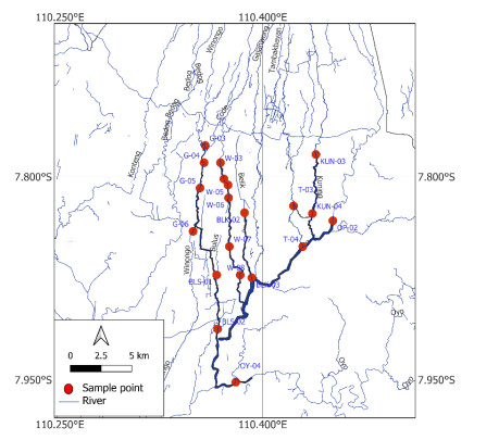
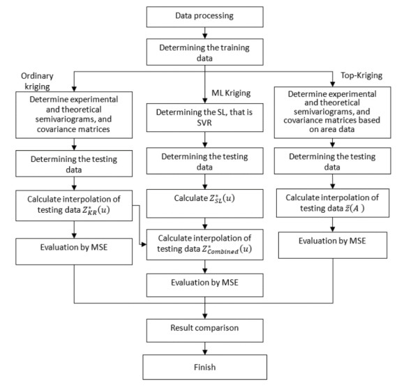
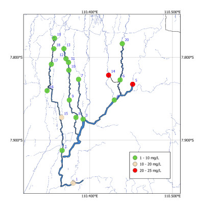
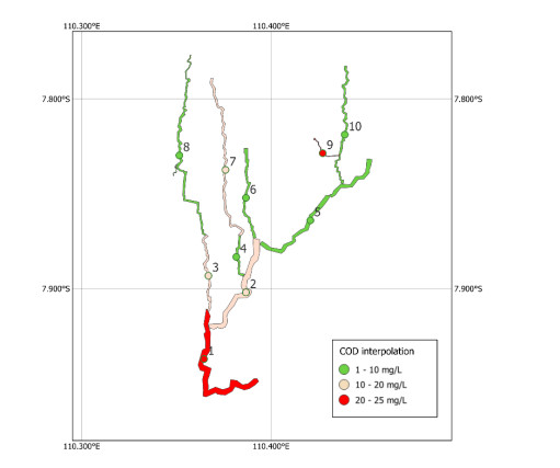
Monitoring of river water quality data is crucial to prevent river water pollution. With limited sampling data, the statistical method of kriging interpolation is indispensable. This method can predict unsampled values based on interconnected surrounding values. Two types of kriging methods that can be applied are Machine Learning (ML) kriging and topological kriging (top-kriging). ML kriging is an extension of ordinary kriging by adding a Super Learning (SL) component. Here, we used SL type Support Vector Regression (SVR). Ordinary Kriging and ML Kriging are based on point values. Top-Kriging is defined as the estimation of streamflow-related variables in ungauged catchments and is based on a non-zero catchment area, not a point value. The three methods were applied in Chemical Oxygen Demand (COD) as water river quality in the Special Region of Yogyakarta (DIY), Indonesia. Based on the Mean Square Error (MSE) and Mean Absolute Error (MAE) comparison, Top kriging provided better accuracy that produced the smallest MSE and MAE. This showed that top kriging is suitable for interpolating data with river flow cases. The interpolation result was that the COD value in the upstream area was low, meaning that the level of organic pollution was minimal. Further downstream, after passing through densely populated residential and industrial areas, the COD values were higher.

| [1] |
Lee J, Lee S, Yu S, et al. (2016) Relationships between water quality parameters in rivers and lakes: BOD 5, COD, NBOPs, and TOC. Environ Monit Assess 188: 1–8. https://doi.org/10.1007/s10661-016-5251-1 doi: 10.1007/s10661-016-5251-1

|
| [2] |
Aboyitungiye JB, Gravitiani E (2021) River pollution and human health risks: Assessment in the locality areas proximity of Bengawan Solo river, Surakarta, Indonesia. Indonesian J Environ Manage Sust 5: 13–20. https://doi.org/10.26554/ijems.2021.5.1.13-20 doi: 10.26554/ijems.2021.5.1.13-20
|
| [3] |
Suphawan K, Chaisee K (2021) Gaussian process regression for predicting water quality index: A case study on Ping River basin, Thailand. AIMS Environ Sci 8: 268–282. https://doi.org/10.3934/environsci.2021018 doi: 10.3934/environsci.2021018
|
| [4] |
Novianta MA, Warsito B, Rachmawati S (2024) Monitoring river water quality through predictive modeling using artificial neural networks backpropagation. AIMS Environ Sci 11: 649–664. https://doi.org/10.3934/environsci.2024032 doi: 10.3934/environsci.2024032
|
| [5] |
Rosyida N, Dinira L, Rusydi AN, et al. (2022) Development of web-based geographic information system for water quality monitoring of watershed in Malang. INTENSIF: Jurnal Ilmiah Penelitian Dan Penerapan Teknologi Sistem Informasi 6: 184–197. https://doi.org/10.29407/intensif.v6i2.17514 doi: 10.29407/intensif.v6i2.17514
|
| [6] | Aneesh PC, Thomas RM (2024) Assessment and mapping of seasonal variation in water quality of Periyar River, Kerala, India. J Comput Sci 17: 1549–3636. |
| [7] |
Raman RK, Bhor M, Manna RK, et al. (2023) Statistical and geostatistical modelling approach for spatio-temporal assessment of river water quality: A case study from lower stretch of River Ganga. Environ Dev Sustain 25: 9963–9989. https://doi.org/10.1007/s10668-022-02472-7 doi: 10.1007/s10668-022-02472-7
|
| [8] | Matheron G (1963) Principles of geostatistics. Econ Geol 58: 1246–1266. |
| [9] |
Chen YC, Yeh HC, Wei C (2012). Estimation of river pollution index in a tidal stream using kriging analysis. Int J Env Res Pub He 9: 3085–3100. https://doi.org/10.3390/ijerph9093085 doi: 10.3390/ijerph9093085
|
| [10] | Bekti RD, Irwansyah E, Kanigoro B, et al. (2018) Ordinary kriging and spatial autocorrelation identification to predict peak ground acceleration in Banda Aceh City, Indonesia, In Applied Computational Intelligence and Mathematical Methods: Computational Methods in Systems and Software 2017, Springer International Publishing, 2: 318–325. https://doi.org/10.1007/978-3-319-67621-0_29 |
| [11] |
Khan M, Almazah MM, EIlahi A, et al. (2023). Spatial interpolation of water quality index based on ordinary kriging and Universal kriging. Geomat Nat Haz Risk 14: 2190853. https://doi.org/10.1080/19475705.2023.2190853 doi: 10.1080/19475705.2023.2190853
|
| [12] |
Marthadyanti A, Harisuseso D, Suhartanto E (2024) Mapping of design rainfall distribution at multiple periods using spatial interpolation in Widas Sub-Watershed, Nganjuk Regency. Jurnal Teknologi dan Rekayasa Sumber Daya Air 4: 450–459. https://doi.org/10.21776/ub.jtresda.2024.004.01.038 doi: 10.21776/ub.jtresda.2024.004.01.038
|
| [13] |
Kethireddy SR, Adegoye GA, Tchounwou PB, et al. (2018) The status of geo-environmental health in Mississippi: Application of spatiotemporal statistics to improve health and air quality. AIMS Environ Sci 5: 273–293. https://doi.org/10.3934/environsci.2018.4.273 doi: 10.3934/environsci.2018.4.273
|
| [14] |
Fahimah N, Salami IR, Oginawati K, et al. (2023) The assessment of water quality and human health risk from pollution of chosen heavy metals in the Upstream Citarum River, Indonesia. J Wate Land Dev 56: 153–163. https://doi.org/10.24425/jwld.2023.143756 doi: 10.24425/jwld.2023.143756
|
| [15] |
Du P, Bai X, Tan K, et al. (2020) Advances of four machine learning methods for spatial data handling: A review. J Geovis Spat Anal 4: 1–25. https://doi.org/10.1007/s41651-020-00048-5 doi: 10.1007/s41651-020-00048-5
|
| [16] |
Erten GE, Yavuz M, Deutsch CV (2022) Combination of machine learning and kriging for spatial estimation of geological attributes. Nat Resour Res 31: 191–213. https://doi.org/10.1007/s11053-021-10003-w doi: 10.1007/s11053-021-10003-w
|
| [17] |
Skøien JO, Merz R, Blöschl G (2006) Top-kriging-geostatistics on stream networks. Hydrol Earth Syst Sc 10: 277–287. https://doi.org/10.5194/hess-10-277-2006 doi: 10.5194/hess-10-277-2006
|
| [18] |
Skøien JO, Blöschl G, Western AW (2003) Characteristic space scales and timescales in hydrology. Water Resour Res 39. https://doi.org/10.1029/2002WR001736 doi: 10.1029/2002WR001736
|
| [19] |
Obaid AN, Mohammed MJ (2020) A comparison of topological kriging and area to point kriging for irregular district area in Iraq. J Mech Con Math Sci 15. https://doi.org/10.26782/jmcms.2020.04.00009 doi: 10.26782/jmcms.2020.04.00009
|
| [20] | Fischer MM, Getis A (2010) Handbook of applied spatial analysis: Software tools, methods and applications, Berlin: Springer, 125–134. |
| [21] | Vapnik V (2013) The nature of statistical learning theory, New York: Springer. |
| [22] |
Balogun AL, Rezaie F, Pham QB, et al. (2021) Spatial prediction of landslide susceptibility in western Serbia using hybrid support vector regression (SVR) with GWO, BAT and COA algorithms. Geosci Front 12: 101104. https://doi.org/10.1016/j.gsf.2020.10.009 doi: 10.1016/j.gsf.2020.10.009
|
| [23] | Rohmadi E, Sekine M, Setiawan B (2022) Impact of slum upgrading to river water quality in Yogyakarta City, Indonesia. Jurnal Teknosains 12: 85–98. |
| [24] |
Brontowiyono W, Asmara AA, Jana R, et al. (2022) Land-use impact on water quality of the opak sub-watershed, Yogyakarta, Indonesia. Sustainability 14: 4346. https://doi.org/10.3390/su14074346 doi: 10.3390/su14074346
|
| [25] |
Archfield SA, Pugliese A, Castellarin A, et al. (2013) Topological and canonical kriging for design flood prediction in ungauged catchments: An improvement over a traditional regional regression approach? Hydrol Earth Syst Sc 17: 1575–1588. https://doi.org/10.5194/hess-17-1575-2013.s doi: 10.5194/hess-17-1575-2013.s
|
Figures(9) / Tables(6)

Rokhana Dwi Bekti, Kris Suryowati, Maria Oktafiana Dedu, Eka Sulistyaningsih, Erma Susanti. Machine learning and topological kriging for river water quality data interpolation[J]. AIMS Environmental Science, 2025, 12(1): 120-136. doi: 10.3934/environsci.2025006


 DownLoad: