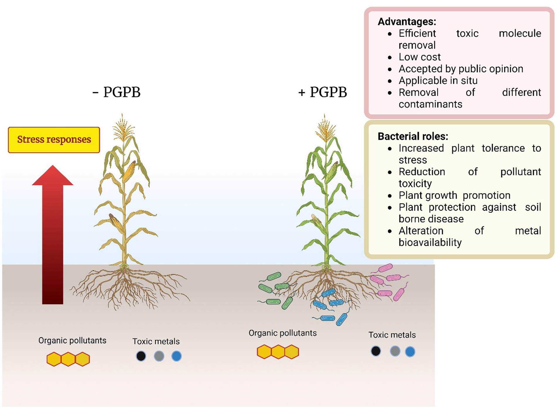
Here, phytoremediation studies of toxic metal and organic compounds using plants augmented with plant growth-promoting bacteria, published in the past few years, were summarized and reviewed. These studies complemented and extended the many earlier studies in this area of research. The studies summarized here employed a wide range of non-agricultural plants including various grasses indigenous to regions of the world. The plant growth-promoting bacteria used a range of different known mechanisms to promote plant growth in the presence of metallic and/or organic toxicants and thereby improve the phytoremediation ability of most plants. Both rhizosphere and endophyte PGPB strains have been found to be effective within various phytoremediation schemes. Consortia consisting of several PGPB were often more effective than individual PGPB in assisting phytoremediation in the presence of metallic and/or organic environmental contaminants.
Citation: Elisa Gamalero, Bernard R. Glick. Use of plant growth-promoting bacteria to facilitate phytoremediation[J]. AIMS Microbiology, 2024, 10(2): 415-448. doi: 10.3934/microbiol.2024021
Here, phytoremediation studies of toxic metal and organic compounds using plants augmented with plant growth-promoting bacteria, published in the past few years, were summarized and reviewed. These studies complemented and extended the many earlier studies in this area of research. The studies summarized here employed a wide range of non-agricultural plants including various grasses indigenous to regions of the world. The plant growth-promoting bacteria used a range of different known mechanisms to promote plant growth in the presence of metallic and/or organic toxicants and thereby improve the phytoremediation ability of most plants. Both rhizosphere and endophyte PGPB strains have been found to be effective within various phytoremediation schemes. Consortia consisting of several PGPB were often more effective than individual PGPB in assisting phytoremediation in the presence of metallic and/or organic environmental contaminants.
1-aminocyclopropane-1-carboxylate
plant growth-promoting bacteria
indole 3-acetic acid
polychlorinated biphenyls
polyaromatic hydrocarbons

| [1] | Fuller R, Landrigan PJ, Balakrishnan K, et al. (2022) Pollution and health. Lancet 6: E535-E547. https://doi.org/10.1016/S2542-5196(22)00090-0 |
| [2] |
Pinhiero HT, MacDonald C, Santos RG, et al. (2018) Rhizobia: From saprophytes to endosymbionts. Nat Rev Microbiol 16: 291-303. https://doi.org/10.1038/nrmicro.2017.171 
|
| [3] |
Nava V, Chandra S, Aherne J, et al. (2023) Plastic debris in lakes and reservoirs. Nature 619: 317-322. https://doi.org/10.1038/s41586-023-06168-4
|
| [4] |
Glick BR (2010) Using soil bacteria to facilitate phytoremediation. Biotechnol Adv 28: 367-374. https://doi.org/10.1016/j.biotechadv.2010.02.001
|
| [5] |
Brookes PC, McGrath SP (1984) Effect of metal toxicity on the size of the soil microbial biomass. Soil Sci 35: 341-346. https://doi.org/10.1111/j.1365-2389.1984.tb00288.x
|
| [6] |
Salt DE, Blaylock M, Kumar NPBA, et al. (1995) Phytoremediation: A novel strategy for the removal of toxic metals from the environment using plants. Nat Biotechnol 13: 468-474. https://doi.org/10.1038/nbt0595-468
|
| [7] | Glick BR (2020) Beneficial Plant-Bacterial Interactions. Heidelberg: Springer 1-383. https://doi.org/10.1007/978-3-030-44368-9 |
| [8] |
Toyama T, Ojima T, Tanaka Y, et al. (2013) Sustainable biodegradation of phenolic endocrine-disrupting chemicals by Phragmites australis-rhizosphere bacteria association. Water Sci Technol 68: 522-529. https://doi.org/10.2166/wst.2013.234
|
| [9] |
Yamaga F, Washio K, Morikawa M (2010) Sustainable biodegradation of phenol by Acinetobacter calcoaceticus P23 isolated from the rhizosphere of duckweed Lemna aoukikusa. Environ Sci Technol 44: 6470-6474. https://doi.org/10.1021/es1007017
|
| [10] |
Ali Z, Waheed H, Kazi AG, et al. (2016) Duckweed: an efficient hyperaccumulator of heavy metals in water bodies. Plant Metal Interaction Emerging Remediation Techniques . Netherlands: Elsevier 411-429. https://doi.org/10.1016/B978-0-12-803158-2.00016-3
|
| [11] |
Khan AU, Khan AN, Waris A, et al. (2022) Phytoremediation of pollutants from wastewater: A concise review. Open Life Sci 13: 488-496. https://doi.org/10.1515/biol-2022-0056
|
| [12] | Glick BR (2012) Plant growth-promoting bacteria: mechanisms and applications. Scientifica 963401. https://doi.org/10.6064/2012/963401 |
| [13] |
Gamalero E, Glick BR (2012) Ethylene and abiotic stress tolerance in plants. Environmental Adaptations and Stress Tolerance of Plants in the Era of Climate Change . Berlin: Springer-Verlag 395-412. https://doi.org/10.1007/978-1-4614-0815-4_18
|
| [14] |
Gepstein S, Glick BR (2013) Strategies to ameliorate abiotic stress-induced plant senescence. Plant Molec Biol 82: 623-633. https://doi.org/10.1007/s11103-013-0038-z
|
| [15] |
Nascimento FX, Rossi MJ, Glick BR (2016) Role of ACC deaminase in stress control of leguminous plants. Plant Growth-Promoting Actinobacteria . Singapore: Springer Science 179-192. https://doi.org/10.1007/978-981-10-0707-1_11
|
| [16] |
Gamalero E, Glick BR (2019) Plant growth-promoting bacteria in agriculture and stressed environments. Modern Soil Microbiology . Florida: CRC Press 361-380. https://doi.org/10.1201/9780429059186-22
|
| [17] | Ali S, Glick BR (2019) Plant-bacterial interactions in management of plant growth under abiotic stresses. New and Future Developments in Microbial Biotechnology and Bioengineering . Netherlands: Elsevier 21-45. https://doi.org/10.1016/B978-0-12-818258-1.00002-9 |
| [18] |
Santoyo G, Gamalero E, Glick BR (2021) Mycorrhizal-bacterial amelioration of plant abiotic and biotic stress. Front Sust Food Sys 5: 672881. https://doi.org/10.3389/fsufs.2021.672881
|
| [19] |
Etesami H, Jeong BR, Glick BR (2023) Potential use of Bacillus spp. as an effective biostimulant against abiotic stress in crops–A review. Curr Res Biotechnol 5: 100128. https://doi.org/10.1016/j.crbiot.2023.100128
|
| [20] |
Glick BR (2003) Phytoremediation: Synergistic use of plants and bacteria to clean up the environment. Biotechnol Adv 21: 383-393. https://doi.org/10.1016/S0734-9750(03)00055-7
|
| [21] |
Vieira FCS, Nahas E (2005) Comparison of microbial numbers in soils by using various culture media and temperatures. Microbiol Res 160: 197-202. https://doi.org/10.1016/j.micres.2005.01.004
|
| [22] |
Hayat R, Ali S, Amara U, Khalid R, et al. (2010) Soil beneficial bacteria and their role in plant growth promotion: a review. Ann Microbiol 60: 579-598. https://doi.org/10.1007/s13213-010-0117-1
|
| [23] |
De Souza R, Ambrosini A, Passaglia LMP (2015) Plant growth-promoting bacteria as inoculants in agricultural soils. Genet Molec Biol 38: 401-419. https://doi.org/10.1590/S1415-475738420150053
|
| [24] |
Glick BR, Gamalero E (2021) Recent developments in the study of plant microbiomes. Microorganisms 9: 1533. https://doi.org/10.3390/microorganisms9071533
|
| [25] |
Walker TS, Bais HP, Grotewold E, et al. (2003) Root exudation and rhizosphere biology. Plant Physiol 132: 44-51. https://doi.org/10.1104/pp.102.019661
|
| [26] |
Canarini A, Kaiser C, Merchant A, et al. (2019) Root exudation of primary metabolites: mechanisms and their roles in plant responses to environmental stimuli. Front Plant Sci 10: 157. https://doi.org/10.3389/fpls.2019.00157
|
| [27] |
Bashir I, War AF, Rafiq I, et al. (2022) Phyllosphere microbiome: diversity and functions. Microbiol Res 254: 126888. https://doi.org/10.1016/j.micres.2021.126888
|
| [28] |
Lindow SE, Brandl MT (2003) Microbiology of the phyllosphere. Appl Environ Microbiol 69: 1875-1883. https://doi.org/10.1128/AEM.69.4.1875-1883.2003
|
| [29] |
Adeleke BS, Babalola OO, Glick BR (2021) Plant growth-promoting root-colonizing bacterial endophytes. Rhizosphere 20: 100433. https://doi.org/10.1016/j.rhisph.2021.100433
|
| [30] |
Ali S, Charles TC, Glick BR (2014) Amelioration of high salinity stress damage by plant growth-promoting bacterial endophytes that contain ACC deaminase. Plant Physiol Biochem 80: 160-167. https://doi.org/10.1016/j.plaphy.2014.04.003
|
| [31] |
Narayanan Z, Glick BR (2022) Secondary metabolites produced by plant bacterial endophytes. Microorg 10: 2008. https://doi.org/10.3390/microorganisms10102008
|
| [32] |
Santoyo G, Moreno-Hagelsieb G, Orozco-Mosqueda MC, et al. (2016) Plant growth-promoting bacterial endophytes. Microbiol Res 183: 92-99. https://doi.org/10.1016/j.micres.2015.11.008
|
| [33] |
Ledermann R, Schulte CCM, Poole PS (2021) How rhizobia adapt to the nodule environment. J Bacteriol 203: e00539-20. https://doi.org/10.1128/JB.00539-20
|
| [34] |
Poole P, Ramachandran V, Terpolilli J (2018) Rhizobia: from saprophytes to endosymbionts. Nat Rev Microbiol 16: 291-303. https://doi.org/10.1038/nrmicro.2017.171
|
| [35] |
Glick BR (1995a) The enhancement of plant growth by free-living bacteria. Can J Microbiol 41: 109-117. https://doi.org/10.1139/m95-015
|
| [36] |
Glick BR (1995b) Metabolic load and heterologous gene expression. Biotechnol Adv 13: 247-261. https://doi.org/10.1016/0734-9750(95)00004-A
|
| [37] |
Gamalero E, Lingua G, Glick BR (2023) Ethylene, ACC, and the plant growth-promoting enzyme ACC deaminase. Biology 12: 1043. https://doi.org/10.3390/biology12081043
|
| [38] |
Reed MLE, Glick BR (2023) The recent use of plant growth-promoting bacteria to promote the growth of agricultural food crops. Agriculture 13: 1089. https://doi.org/10.3390/agriculture13051089
|
| [39] |
Bonfante P, Genre A (2010) Mechanisms underlying beneficial plant-Fungus interactions in mycorrhizal symbiosis. Nat Commun 1: 48. https://doi.org/10.1038/ncomms1046
|
| [40] |
Figueiredo AF, Boy J, Guggenberger G (2021) Common mycorrhizae network: A review of the theories and mechanisms behind underground interactions. Front Fungal Biol 2: 735299. https://doi.org/10.3389/ffunb.2021.735299
|
| [41] |
Brundrett MC (2002) Coevolution of roots and mycorrhizas of land plants. New Phytol 154: 275-304. https://doi.org/10.1046/j.1469-8137.2002.00397.x
|
| [42] |
Bonfante P, Anca IA (2009) Plants, mycorrhizal fungi, and bacteria: A network of interactions. Annu Rev Microbiol 63: 363-383. https://doi.org/10.1146/annurev.micro.091208.073504
|
| [43] |
Chen M, Arato M, Borghi L, et al. (2018) Beneficial services of arbuscular mycorrhizal fungi–from ecology to application. Front Plant Sci 9: 1270. https://doi.org/10.3389/fpls.2018.01270
|
| [44] |
Frey-Klett P, Garbaye J, Tarkka M (2007) The mycorrhiza helper bacteria revisited. New Phytol 176: 22-36. https://doi.org/10.1111/j.1469-8137.2007.02191.x
|
| [45] |
Liu S, Yang B, Liang Y, et al. (2020) Prospect of phytoremediation combined with other approaches for remediation of heavy metal-polluted soils. Environ Sci Pollut Res 27: 16069-16085. https://doi.org/10.1007/s11356-020-08282-6
|
| [46] |
Raffa CM, Chiampo F, Shanthakumar S (2021) Remediation of Metal/Metalloid-polluted soils: a short review. Appl Sci 11: 4134. https://doi.org/10.3390/app11094134
|
| [47] |
Rajendran S, Priya TAK, Khoo KS, et al. (2021) A critical review on various remediation approaches for heavy metal contaminants removal from contaminated soils. Chemosphere 287: 132369. https://doi.org/10.1016/j.chemosphere.2021.132369
|
| [48] |
Raklami A, Meddich A, Oufdou K, et al. (2022) Plants—Microorganisms-based bioremediation for heavy metal cleanup: recent developments, phytoremediation techniques, regulation mechanisms, and molecular responses. Int J Mol Sci 23: 5031. https://doi.org/10.3390/ijms23095031
|
| [49] |
Alves ARA, Yin Q, Oliveira RS, et al. (2022) Plant growth-promoting bacteria in phytoremediation of metal-polluted soils: Current knowledge and future directions. Sci Tot Environ 838: 156435. https://doi.org/10.1016/j.scitotenv.2022.156435
|
| [50] |
Pande V, Pandey SC, Sati D, et al. (2022) Microbial interventions in bioremediation of heavy metal contaminants in agroecosystem. Front Microbiol 6: 824084. https://doi.org/10.3389/fmicb.2022.824084
|
| [51] |
Jain D, Kour R, Bhojiya AA, et al. (2020) Zinc tolerant plant growth promoting bacteria alleviates phytotoxic effects of zinc on maize through zinc immobilization. Sci Rep 10: 13865. https://doi.org/10.1038/s41598-020-70846-w
|
| [52] |
Saeed Q, Xiukang W, Haider FU, et al. (2021) Rhizosphere bacteria in plant growth promotion, biocontrol, and bioremediation of contaminated sites: a comprehensive review of effects and mechanisms. Int J Mol Sci 22: 10529. https://doi.org/10.3390/ijms221910529
|
| [53] |
Clavero-León C, Ruiz D, Cillero J, et al. (2021) The multi metal-resistant bacterium Cupriavidus metallidurans CH34 affects growth and metal mobilization in Arabidopsis thaliana plants exposed to copper. Peer J 9: e11373. https://doi.org/10.7717/peerj.11373
|
| [54] | Adiloğlu S, Açikgöz FE, Gürgan M (2021) Use of phytoremediation for pollution removal of hexavalent chromium-contaminated acid agricultural soils. Global NEST J 23: 400-406. https://doi.org/10.30955/gnj.003433 |
| [55] |
Li Y, Mo L, Zhou X, et al. (2021) Characterization of plant growth-promoting traits of Enterobacter sp. and its ability to promote cadmium/lead accumulation in Centella asiatica L. Environ Sci Pollut Res Int 29: 4101-4115. https://doi.org/10.1007/s11356-021-15948-2
|
| [56] |
Sangsuwan P, Prapagdee B (2021) Cadmium phytoremediation performance of two species of Chlorophytum and enhancing their potentials by cadmium-resistant bacteria. Environ Technol Innov 21: 101311. https://doi.org/10.1016/j.eti.2020.101311
|
| [57] |
Peng PH, Liang K, Luo H, et al. (2021) A Bacillus and Lysinibacillus sp. bio-augmented Festuca arundinacea phytoremediation system for the rapid decontamination of chromium influenced soil. Chemosphere 283: 131186. https://doi.org/10.1016/j.chemosphere.2021.131186
|
| [58] |
Kumar A, Tripti, Voropaeva O, et al. (2021) Bioaugmentation with copper tolerant endophyte Pseudomonas lurida strain EOO26 for improved plant growth and copper phytoremediation by Helianthus annuus. Chemosphere 266: 128983. https://doi.org/10.1016/j.chemosphere.2020.128983
|
| [59] |
Tirry N, Kouchou A, El Omari B, et al. (2021) Improved chromium tolerance of Medicago sativa by plant growth-promoting rhizobacteria (PGPR). J Genetic Engin Biotechnol 19: 149. https://doi.org/10.1186/s43141-021-00254-8
|
| [60] |
Wang Y, Yang R, Hao J, et al. (2021) The impact of Pseudomonas monteilii PN1 on enhancing the alfalfa phytoextraction and responses of rhizosphere soil bacterial communities in cadmium-contaminated soil. J Environ Chem Eng 9: 106533. https://doi.org/10.1016/j.jece.2021.106533
|
| [61] |
Liu S, Liu H, Chen R, et al. (2021) Role of two plant growth-promoting bacteria in remediating cadmium-contaminated soil combined with Miscanthus floridulus (Lab.). Plants 10: 912. https://doi.org/10.3390/plants10050912
|
| [62] |
Yankey R, Karanja JK, Okal EJ, et al. (2021) A consortium of plant growth-promoting rhizobacteria strains synergistically assists Jujuncao (Pennisetum giganteum) to remediate cadmium contaminated soils. Appl Ecol Environ Res 19: 2425-2442. https://doi.org/10.15666/aeer/1903_24252442
|
| [63] |
Abou-Shanab RAI, Santelli CM, Sadowsky MJ (2021) Bioaugmentation with As-transforming bacteria improves arsenic availability and uptake by the hyperaccumulator plant Pteris vittate (L). Int J Phytorem 24: 420-428. https://doi.org/10.1080/15226514.2021.1951654
|
| [64] |
Niu XY, Wang SK, Zhou J, et al. (2021) Inoculation with indigenous rhizosphere microbes enhances aboveground accumulation of lead in Salix integra Thunb. by improving transport coefficients. Front Microbiol 12: 686812. https://doi.org/10.3389/fmicb.2021.686812
|
| [65] |
Zainab N, Amna Khan AA, Azeem MA, et al. (2021) PGPR-mediated Plant Growth attributes and metal extraction ability of Sesbania sesban L. in industrially contaminated soils. Agronomy 11: 1820. https://doi.org/10.3390/agronomy11091820
|
| [66] |
Llimós M, Bistué M, Marcelino J, et al. (2021) A native Zn-solubilising bacterium from mine soil promotes plant growth and facilitates phytoremediation. J Soils Sed 21: 2301-2314. https://doi.org/10.1007/s11368-021-02934-x
|
| [67] |
Tanwir K, Javed MT, Abbas S, et al. (2021) Serratia sp. CP-13 alleviates Cd toxicity by morpho-physio-biochemical improvements, antioxidative potential and diminished Cd uptake in Zea mays L. cultivars differing in Cd tolerance. Ecotoxicol Environ Saf 208: 111584. https://doi.org/10.1016/j.ecoenv.2020.111584
|
| [68] |
Franchi E, Barbafieri M, Petruzzelli G, et al. (2022) Improvement of Arsenic phytoextraction using indigenous bacteria and mobilizing agents. Appl Sci 12: 9059. https://doi.org/10.3390/app12189059
|
| [69] |
Ustiatik R, Nuraini Y, Suharjono S, et al. (2022) Endophytic bacteria promote biomass production and mercury-bioaccumulation of Bermuda grass and Indian goosegrass. Int J Phytorem 24: 1184-1192. https://doi.org/10.1080/15226514.2021.2023461
|
| [70] |
Ma J, Alshaya H, Okla MK, et al. (2022) Application of cerium dioxide nanoparticles and chromium-resistant bacteria reduced chromium toxicity in sunflower plants. Front Plant Sci 13: 876119. https://doi.org/10.3389/fpls.2022.876119
|
| [71] |
Wei Xie L, Yang R, Liu B, et al. (2022) Effects of Pb-, Cd-resistant bacterium Pantoea sp. on growth, heavy metal uptake and bacterial communities in oligotrophic growth substrates of Lolium multiflorum Lam. Environ Sci Pollut Res Int 29: 50742-50754. https://doi.org/10.1007/s11356-022-19180-4
|
| [72] |
Alka S, Shahir S, Ibrahim N, et al. (2023) Assessment of plant growth promotion properties and impact of Microbacterium foliorum for arsenic removal in Melastoma malabathricum. Biorem J 27: 251-262. https://doi.org/10.1080/10889868.2022.2048629
|
| [73] |
Liu A, Wang W, Zheng X, et al. (2022) Improvement of the Cd and Zn phytoremediation efficiency of rice (Oryza sativa) through the inoculation of a metal-resistant PGPR strain. Chemosphere 302: 134900. https://doi.org/10.1016/j.chemosphere.2022.134900
|
| [74] |
Liu C, Li B, Dong Y, et al. (2022) Endophyte colonization enhanced cadmium phytoremediation by improving endosphere and rhizosphere microecology characteristics. J Hazard Mater 15: 128829. https://doi.org/10.1016/j.jhazmat.2022.128829
|
| [75] |
Das PK, Das BP, Dash P (2022) A super-tolerant bacteria strain improves phytoremediation of Cr (VI) contaminated soil with Pongamia pinnata. Rhizosphere 22: 100543. https://doi.org/10.1016/j.rhisph.2022.100543
|
| [76] |
Du S, Lu Q, Liu L, et al. (2022) Rhodococcus qingshengii facilitates the phytoextraction of Zn, Cd, Ni, and Pb from soils by Sedum alfredii Hance. J Hazard Mater 15: 127638. https://doi.org/10.1016/j.jhazmat.2021.127638
|
| [77] |
Ma L, Huang L, Liu Q, et al. (2022) Positive effects of applying endophytic bacteria in eggplant-Sedum intercropping system on Cd phytoremediation and vegetable production in cadmium polluted greenhouse. J Environ Sci 115: 383-391. https://doi.org/10.1016/j.jes.2021.08.005
|
| [78] |
Cheng X, Cao X, Tan C, et al. (2022) Effects of four endophytic bacteria on cadmium speciation and remediation efficiency of Sedum plumbizincicola in farmland soil. Environ Sci Pollut Res Int 29: 89557-89569. https://doi.org/10.1007/s11356-022-21711-y
|
| [79] |
Chi Y, You Y, Wang J, et al. (2022) Two plant growth-promoting bacterial Bacillus strains possess different mechanisms in affecting cadmium uptake and detoxification of Solanum nigrum L. Chemosphere 305: 135488. https://doi.org/10.1016/j.chemosphere.2022.135488
|
| [80] |
Zhang Y, Zhao S, Liu S, et al. (2022) Enhancing the phytoremediation of heavy metals by combining hyperaccumulator and heavy metal-resistant plant growth-promoting bacteria. Front Plant Sci 13: 912350. https://doi.org/10.3389/fpls.2022.912350
|
| [81] |
Vishnupradeep R, Benedict Bruno L, Taj Z, et al. (2022) Plant growth promoting bacteria improve growth and phytostabilization potential of Zea mays under chromium and drought stress by altering photosynthetic and antioxidant responses. Environ Technol Innov 25: 102154. https://doi.org/10.1016/j.eti.2021.102154
|
| [82] |
Wu Q, Lin X, Li S (2023) Endophytic Bacillus sp. AP10 harboured in Arabis paniculata mediates plant growth promotion and manganese detoxification. Ecotoxicol Environ Saf 262: 115170. https://doi.org/10.1016/j.ecoenv.2023.115170
|
| [83] |
Kumar H, Ishtiyaq S, Favas PJC, et al. (2023) Effect of metal-resistant PGPB on the metal uptake, antioxidative defense, physiology, and growth of Atriplex lentiformis (Torr.) S.Wats. in soil contaminated with Cadmium and Nickel. J Plant Growth Regul 42: 3868-3887. https://doi.org/10.1007/s00344-022-10853-5
|
| [84] |
Liu H, Huang H, Xie Y, et al. (2023) Integrated biochemical and transcriptomic analysis reveals the effects of Burkholderia sp. SRB-1 on cadmium accumulating in Chrysopogon zizanioides L. under Cd stress. J Environ Manag 1: 117723. https://doi.org/10.1016/j.jenvman.2023.117723
|
| [85] | Yang D, Zuo M, Chen Y, et al. (2023) Effects of the promoting bacterium on growth of plant under cadmium stress. Intern J Phytorem 8: 1-10. https://doi.org/10.1080/15226514.2023.2241925 |
| [86] |
Jin J, Mi R, Li Q, et al. (2023) Bacillus thuringiensis enhances the ability of ryegrass to remediate cadmium-contaminated soil. Sustainability 15: 5177. https://doi.org/10.3390/su15065177
|
| [87] |
Gao T, Liu Y, Yang D, et al. (2023) Inoculation of exogenous complex bacteria to enhance resistance in alfalfa and combined remediation of heavy metal-contaminated soil. Curr Microbiol 16: 213. https://doi.org/10.1007/s00284-023-03299-9
|
| [88] |
Wang X, Luo S, Chen Y, et al. (2023) Potential of Miscanthus floridulus associated with endophytic bacterium Bacillus cereus BL4 to remediate cadmium contaminated soil. Sci Tot Environ 20: 159384. https://doi.org/10.1016/j.scitotenv.2022.159384
|
| [89] |
Muratova A, Golubev S, Romanova V, et al. (2023) Effect of heavy-metal-resistant PGPR inoculants on growth, rhizosphere microbiome and remediation potential of Miscanthus giganteus in zinc-contaminated soil. Microorganisms 11: 1516. https://doi.org/10.3390/microorganisms11061516
|
| [90] | Houida S, Yakkou L, Kaya LO, et al. (2023) Plant growth-promoting bacteria isolated from earthworms enhance spinach growth and its phytoremediation potential in metal-contaminated soils. Int Microbiol 29: 37516695. https://doi.org/10.1007/s10123-023-00402-9 |
| [91] |
He T, Xu ZM, Wang JF, et al. (2023) Inoculation of Escherichia coli enriched the key functional bacteria that intensified cadmium accumulation by halophyte Suaeda salsa in saline soils. J Haz Mater 15: 131922. https://doi.org/10.1016/j.jhazmat.2023.131922
|
| [92] |
Mohanty M, Mohapatra S (2023) Synergistic effect of PGPR and PSB for alleviation of chromium toxicity in Vigna radiata (L.) R. Wilczek seedlings. Int J Phytorem 25: 1733-1742. https://doi.org/10.1080/15226514.2023.2189479
|
| [93] |
Rojas-Solis D, García Rodríguez YM, Larsen J, et al. (2023) Growth promotion traits and emission of volatile organic compounds of two bacterial strains stimulate growth of maize exposed to heavy metals. Rhizosphere 27. https://doi.org/10.1016/j.rhisph.2023.100739
|
| [94] | Kumar B, Verma VK, Singh SK, et al. (2014) Polychlorinated biphenyls in residential soils and their health risk and hazard in an industrial city in India. J Public Health Res 1: 252. https://doi.org/10.4081/jphr.2014.252 |
| [95] |
Bisht S, Pandey P, Bhargava B, et al. (2015) Bioremediation of polyaromatic hydrocarbons (PAHs) using rhizosphere technology. Braz J Microbiol 1: 7-21. https://doi.org/10.1590/S1517-838246120131354
|
| [96] |
Ancona V, Barra Caracciolo A, Grenni P, et al. (2017) Plant-assisted bioremediation of a historically PCB and heavy metal-contaminated area in Southern Italy. N Biotechnol 25: 65-73. https://doi.org/10.1016/j.nbt.2016.09.006
|
| [97] |
Ancona V, Rascio I, Aimola G (2021) Poplar-assisted bioremediation for recovering a PCB and Heavy-Metal-contaminated area. Agriculture 11: 689. https://doi.org/10.3390/agriculture11080689
|
| [98] |
Gabriele I, Race M, Papirio S, et al. (2021) Phytoremediation of pyrene-contaminated soils: A critical review of the key factors affecting the fate of pyrene. J Environ Manag 293: 112805. https://doi.org/10.1016/j.jenvman.2021.112805
|
| [99] |
Kafle A, Timilsina A, Gautam A, et al. (2022) Phytoremediation: mechanisms, plant selection and enhancement by natural and synthetic agents. Environ Adv 8: 100203. https://doi.org/10.1016/j.envadv.2022.100203
|
| [100] |
Schwitzguébel JP (2017) Phytoremediation of soils contaminated by organic compounds: hype, hope and facts. J Soils Sed 17: 1492-1502. https://doi.org/10.1007/s11368-015-1253-9
|
| [101] |
Gamalero E, Glick BR (2015) Bacterial modulation of plant ethylene levels. Plant Physiol 169: 13-22. https://doi.org/10.1104/pp.15.00284
|
| [102] |
Vocciante M, Grifoni M, Fusini D, et al. (2022) The role of Plant Growth-Promoting Rhizobacteria (PGPR) in mitigating plant's environmental stresses. Appl Sci 12: 1231. https://doi.org/10.3390/app12031231
|
| [103] |
Guan C, Fu W, Zhang X, et al. (2023) Enhanced phytoremediation efficiency of PHE-contaminated soil by rape (Brassica napus L.) assisted with PHE-degradable PGPR through modulating rhizobacterial communities. Ind Crops Prod 202: 117057. https://doi.org/10.1016/j.indcrop.2023.117057
|
| [104] |
Siciliano SD, Fortin N, Mihoc A, et al. (2001) Selection of specific endophytic bacterial genotypes by plants in response to soil contamination. Appl Environ Microbiol 67: 2469-2475. https://doi.org/10.1128/AEM.67.6.2469-2475.2001
|
| [105] |
Afzal M, Khan QM, Sessitsch A (2014) Endophytic bacteria: prospects and applications for the phytoremediation of organic pollutants. Chemosphere 117: 232-242. https://doi.org/10.1016/j.chemosphere.2014.06.078
|
| [106] |
Karaś MA, Wdowiak-Wróbel S, Sokołowski W (2021) Selection of endophytic strains for enhanced bacteria-assisted phytoremediation of organic pollutants posing a public health hazard. Int J Mol Sci 3: 9557. https://doi.org/10.3390/ijms22179557
|
| [107] |
Tiwari P, Bae H (2020) Horizontal gene transfer and endophytes: an implication for the acquisition of novel traits. Plants 9: 305. https://doi.org/10.3390/plants9030305
|
| [108] |
Li N, Liu R, Chen J, et al. (2021) Enhanced phytoremediation of PAHs and cadmium contaminated soils by a Mycobacterium. Sci Tot Environ 1: 141198. https://doi.org/10.1016/j.scitotenv.2020.141198
|
| [109] |
Kotoky R, Pandey P (2021) The genomic attributes of Cd-resistant, hydrocarbonoclastic Bacillus subtilis SR1 for rhizodegradation of benzo(a)pyrene under co-contaminated conditions. Genomics 113: 613-623. https://doi.org/10.1016/j.ygeno.2020.09.057
|
| [110] |
Sun L, Zhu G, Liao X (2021) Rhizosphere interactions between PAH-degrading bacteria and Pteris vittata L. on arsenic and phenanthrene dynamics and transformation. Chemosphere 285: 131415. https://doi.org/10.1016/j.chemosphere.2021.131415
|
| [111] |
Ali MH, Khan MI, Bashir S, et al. (2021) Biochar and Bacillus sp. MN54 assisted phytoremediation of diesel and plant growth promotion of maize in hydrocarbons contaminated soil. Agronomy 11: 1795. https://doi.org/10.3390/agronomy11091795
|
| [112] |
Hussain F, Khan AHA, Hussain I (2022) Soil conditioners improve rhizodegradation of aged petroleum hydrocarbons and enhance the growth of Lolium multiflorum. Environ Sci Pollut Res 29: 9097-9109. https://doi.org/10.1007/s11356-021-16149-7
|
| [113] |
Bhuyan B, Kotoky R, Pandey P (2023) Impacts of rhizoremediation and biostimulation on soil microbial community, for enhanced degradation of petroleum hydrocarbons in crude oil-contaminated agricultural soils. Environ Sci Pollut Res 30: 94649-94668. https://doi.org/10.1007/s11356-023-29033-3
|
| [114] |
Singh K, Tripathi S, Chandra R (2023) Bacterial assisted phytoremediation of heavy metals and organic pollutants by Cannabis sativa as accumulator plants growing on distillery sludge for ecorestoration of polluted site. J Environ Manag 332: 117294. https://doi.org/10.1016/j.jenvman.2023.117294
|
| [115] |
Li W, Li WB, Xing LJ (2023) Effect of arbuscular mycorrhizal fungi (AMF) and plant growth-promoting rhizobacteria (PGPR) on microorganism of phenanthrene and pyrene contaminated soils. Int J Phytorem 25: 240-251. https://doi.org/10.1080/15226514.2022.2071832
|
| [116] |
Gao M, Gao B, Zhang X, et al. (2022) Effects of Plant Growth–Promoting Rhizobacteria (PGPR) on the phytoremediation of pyrene-nickel-contaminated soil by Juncus effusus. Water Air Soil Pollut 233: 458. https://doi.org/10.1007/s11270-022-05933-x
|
| [117] |
Rafique HM, Khan MY, Asghar HN, et al. (2023) Converging alfalfa (Medicago sativa L.) and petroleum hydrocarbon acclimated ACC-deaminase containing bacteria for phytoremediation of petroleum hydrocarbon contaminated soil. Int J Phytorem 25: 717-727. https://doi.org/10.1080/15226514.2022.2104214
|
| [118] |
ShirzadianGilan R, Parvizi Y, Pazira E, et al. (2023) Remediation capacity of drought-tolerant plants and bacteria in petroleum hydrocarbon-contaminated soil in Iran. South Afr J Bot 153: 1-10. https://doi.org/10.1016/j.sajb.2022.12.014
|
| [119] |
Cui C, Shen J, Zhu Y, et al. (2023) Bioremediation of phenanthrene in saline-alkali soil by biochar-immobilized moderately halophilic bacteria combined with Suaeda salsa L. Sci Tot Environ 1: 163279. https://doi.org/10.1016/j.scitotenv.2023.163279
|
| [120] |
Ali MH, Khan MI, Naveed M, et al. (2023) Microbe-assisted rhizodegradation of hydrocarbons and growth enhancement of wheat plants in hydrocarbons contaminated soil. Int J Environ Sci Technol 21: 3169-3184. https://doi.org/10.1007/s13762-023-05174-3
|
| [121] |
Yang KM, Poolpak T, Pokethitiyook P, et al. (2022) Assessment of dynamic microbial community structure and rhizosphere interactions during bioaugmented phytoremediation of petroleum contaminated soil by a newly designed rhizobox system. Int J Phytorem 24: 1505-1517. https://doi.org/10.1080/15226514.2022.2040420
|
| [122] |
Wojtowicz K, Steliga T, Kapusta P, et al. (2023) Oil-contaminated soil remediation with biodegradation by autochthonous microorganisms and phytoremediation by maize (Zea mays). Molecules 17: 6104. https://doi.org/10.3390/molecules28166104
|
Figures(4) / Tables(2)

Elisa Gamalero, Bernard R. Glick. Use of plant growth-promoting bacteria to facilitate phytoremediation[J]. AIMS Microbiology, 2024, 10(2): 415-448. doi: 10.3934/microbiol.2024021


 DownLoad: