In this paper we study the existence of solutions of the Dirichlet problem associated to the following nonlinear PDE
$ \begin{equation*} { } -{{{\rm{\;div}}}}\big(a(x)\,\nabla u|\nabla u|^{p-2}\big) -{{{\rm{\;div}}}}\big( |u|^{(r-1)\lambda+1}\nabla u|\nabla u|^{\lambda-2}\big) = f \end{equation*} $
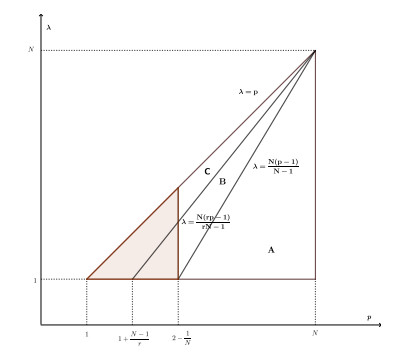
where $ 1 < \lambda \leq p $, $ r > 1 $ and $ f \in L^1(\Omega) $.
Citation: Lucio Boccardo, Giuseppa Rita Cirmi. Regularizing effect in some Mingione’s double phase problems with very singular data[J]. Mathematics in Engineering, 2023, 5(3): 1-15. doi: 10.3934/mine.2023069
In this paper we study the existence of solutions of the Dirichlet problem associated to the following nonlinear PDE
$ \begin{equation*} { } -{{{\rm{\;div}}}}\big(a(x)\,\nabla u|\nabla u|^{p-2}\big) -{{{\rm{\;div}}}}\big( |u|^{(r-1)\lambda+1}\nabla u|\nabla u|^{\lambda-2}\big) = f \end{equation*} $
where $ 1 < \lambda \leq p $, $ r > 1 $ and $ f \in L^1(\Omega) $.

| [1] |
D. Arcoya, L. Boccardo, Regularizing effect of the interplay between coefficients in some elliptic equations, J. Funct. Anal., 268 (2015), 1153–1166. https://doi.org/10.1016/j.jfa.2014.11.011 doi: 10.1016/j.jfa.2014.11.011

|
| [2] |
P. Baroni, M. Colombo, G. Mingione, Harnack inequalities for double phase functionals, Nonlinear Anal., 121 (2015), 206–222. https://doi.org/10.1016/j.na.2014.11.001 doi: 10.1016/j.na.2014.11.001
|
| [3] |
P. Baroni, M. Colombo, G. Mingione, Regularity for general functionals with double phase, Calc. Var., 57 (2018), 62. https://doi.org/10.1007/s00526-018-1332-z doi: 10.1007/s00526-018-1332-z
|
| [4] | P. Bénilan, L. Boccardo, T. Gallouët, R. Gariepy, M. Pierre, J. L. Vazquez, An $L^1$ theory of existence and uniqueness of solutions of nonlinear elliptic equations, Ann. Scuola Norm. Sci., 22 (1995), 241–273. |
| [5] | L. Boccardo, Some nonlinear Dirichlet problems in $L^1$ involving lower order terms in divergence form, In: Progress in elliptic and parabolic partial differential equations, Harlow: Longman, 1996, 43–57. |
| [6] |
L. Boccardo, G. R. Cirmi, Some elliptic equations with $W_0^{1, 1}$ solutions, Nonlinear Anal., 153 (2017), 130–141. https://doi.org/10.1016/j.na.2016.09.007 doi: 10.1016/j.na.2016.09.007
|
| [7] |
L. Boccardo, T. Gallouët, Nonlinear elliptic and parabolic equations involving measure data, J. Funct. Anal., 87 (1989), 149–169. https://doi.org/10.1016/0022-1236(89)90005-0 doi: 10.1016/0022-1236(89)90005-0
|
| [8] |
L. Boccardo, T. Gallouët, Nonlinear elliptic equations with right hand side measures, Commun. Part. Diff. Eq., 17 (1992), 189–258. https://doi.org/10.1080/03605309208820857 doi: 10.1080/03605309208820857
|
| [9] |
L. Boccardo, T. Gallouët, Strongly nonlinear elliptic equations having natural growth terms and $L^1-$ data, Nonlinear Anal., 19 (1992), 573–579. https://doi.org/10.1016/0362-546X(92)90022-7 doi: 10.1016/0362-546X(92)90022-7
|
| [10] |
H. Brézis, W. A. Strauss, Semi-linear second-order elliptic equations in $L^1$, J. Math. Soc. Japan, 25 (1973), 565–590. https://doi.org/10.2969/jmsj/02540565 doi: 10.2969/jmsj/02540565
|
| [11] |
G. R. Cirmi, Regularity of the solutions to nonlinear elliptic equations with a lower-order term, Nonlinear Anal., 25 (1995), 569–580. https://doi.org/10.1016/0362-546X(94)00173-F doi: 10.1016/0362-546X(94)00173-F
|
| [12] |
M. Colombo, G. Mingione, Bounded minimisers of double phase variational integrals, Arch. Rational Mech. Anal., 218 (2015), 219–273. https://doi.org/10.1007/s00205-015-0859-9 doi: 10.1007/s00205-015-0859-9
|
| [13] |
M. Colombo, G. Mingione, Regularity for double phase variational problems, Arch. Rational Mech. Anal., 215 (2015), 443–496. https://doi.org/10.1007/s00205-014-0785-2 doi: 10.1007/s00205-014-0785-2
|
| [14] | C. De Filippis, G. Mingione, Nonuniformly elliptic Schauder theory, arXiv: 2201.07369. |
| [15] |
J. Leray, J. L. Lions, Quelques résultats de Višik sur les problèmes elliptiques semi-linéaires par les méthodes de Minty et Browder, Bull. Soc. Math. France, 93 (1965), 97–107. https://doi.org/10.24033/bsmf.1617 doi: 10.24033/bsmf.1617
|
| [16] |
P. Marcellini, Regularity and existence of solutions of elliptic equations with $p, q$-growth conditions, J. Differ. Equations, 90 (1991), 1–30. https://doi.org/10.1016/0022-0396(91)90158-6 doi: 10.1016/0022-0396(91)90158-6
|
| [17] |
P. Marcellini, Local Lipschitz continuity for $p, q$-PDEs with explicit $u$-dependence, Nonlinear Anal., 226 (2023), 113066. https://doi.org/10.1016/j.na.2022.113066 doi: 10.1016/j.na.2022.113066
|
| [18] |
G. Stampacchia, Le problème de Dirichlet pour les équations elliptiques du second ordre à coefficients discontinus, Ann. Inst. Fourier, 15 (1965), 189–257. https://doi.org/10.5802/aif.204 doi: 10.5802/aif.204
|
Figures(1)

Lucio Boccardo, Giuseppa Rita Cirmi. Regularizing effect in some Mingione’s double phase problems with very singular data[J]. Mathematics in Engineering, 2023, 5(3): 1-15. doi: 10.3934/mine.2023069


 DownLoad: