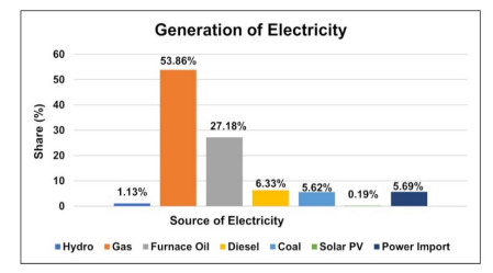
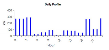
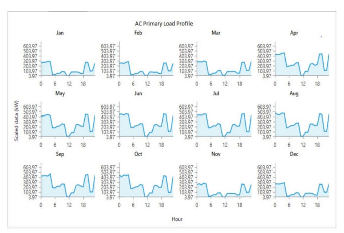
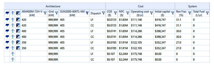
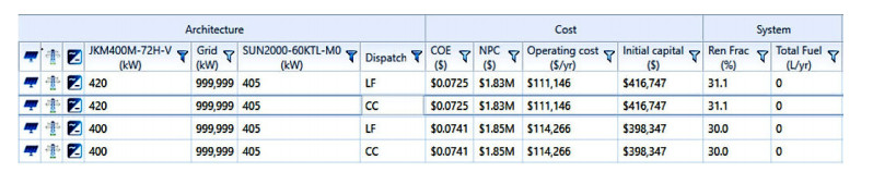
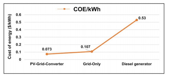
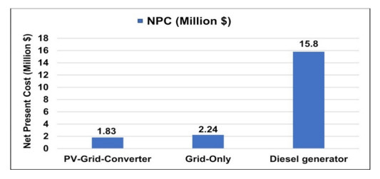
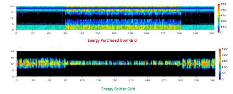
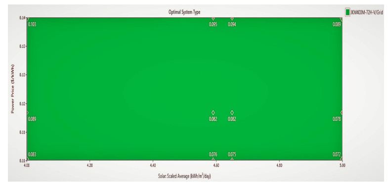
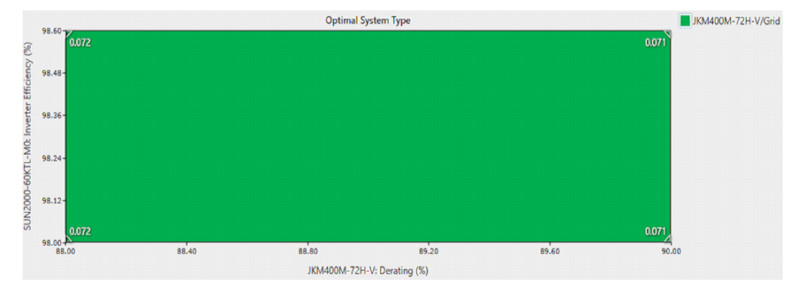
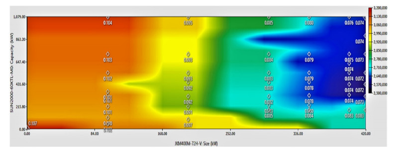
Growing energy demand has exacerbated the issue of energy security and caused us to necessitate the utilization of renewable resources. The best alternative for promoting generation in Bangladesh from renewable energy is solar photovoltaic technology. Grid-connected solar photovoltaic (PV) systems are becoming increasingly popular, considering solar potential and the recent cost of PV modules. This study proposes a grid-connected solar PV system with a net metering strategy using the Hybrid Optimization of Multiple Electric Renewables model. The HOMER model is used to evaluate raw data, to create a demand cycle using data from load surveys, and to find the best cost-effective configuration. A sensitivity analysis was also conducted to assess the impact of differences in radiation from the solar (4, 4.59, 4.65, 5 kWh/m2/day), PV capacity (0 kW, 100 kW, 200 kW, 300 kW, 350 kW, 400 kW, 420 kW), and grid prices ($0.107, $0.118, $0.14 per kWh) upon that optimum configuration. Outcomes reveal that combining 420 kW of PV with a 405-kW converter and connecting to the utility grid is the least expensive and ecologically healthy configuration of the system. The electricity generation cost is estimated to be 0.0725 dollars per kilowatt-hour, and the net present value is 1.83 million dollars with a payback period of 6.4 years based on the system's 20-year lifespan. Also, compared to the existing grid and diesel-generator system, the optimized system, with a renewable fraction of 31.10%, provides a reduction in carbon dioxide emissions of 191 tons and 1,028 tons, respectively, each year.
Citation: Md. Mehadi Hasan Shamim, Sidratul Montaha Silmee, Md. Mamun Sikder. Optimization and cost-benefit analysis of a grid-connected solar photovoltaic system[J]. AIMS Energy, 2022, 10(3): 434-457. doi: 10.3934/energy.2022022
Growing energy demand has exacerbated the issue of energy security and caused us to necessitate the utilization of renewable resources. The best alternative for promoting generation in Bangladesh from renewable energy is solar photovoltaic technology. Grid-connected solar photovoltaic (PV) systems are becoming increasingly popular, considering solar potential and the recent cost of PV modules. This study proposes a grid-connected solar PV system with a net metering strategy using the Hybrid Optimization of Multiple Electric Renewables model. The HOMER model is used to evaluate raw data, to create a demand cycle using data from load surveys, and to find the best cost-effective configuration. A sensitivity analysis was also conducted to assess the impact of differences in radiation from the solar (4, 4.59, 4.65, 5 kWh/m2/day), PV capacity (0 kW, 100 kW, 200 kW, 300 kW, 350 kW, 400 kW, 420 kW), and grid prices ($0.107, $0.118, $0.14 per kWh) upon that optimum configuration. Outcomes reveal that combining 420 kW of PV with a 405-kW converter and connecting to the utility grid is the least expensive and ecologically healthy configuration of the system. The electricity generation cost is estimated to be 0.0725 dollars per kilowatt-hour, and the net present value is 1.83 million dollars with a payback period of 6.4 years based on the system's 20-year lifespan. Also, compared to the existing grid and diesel-generator system, the optimized system, with a renewable fraction of 31.10%, provides a reduction in carbon dioxide emissions of 191 tons and 1,028 tons, respectively, each year.

| [1] | Power system master plan-2016 (2021) Available from: https://powerdivision.gov.bd/site/page/f68eb32d-cc0b-483e-b047-13eb81da6820/Power-System-Master-Plan-2016. |
| [2] |
Nallapaneni MK, Chopra S, Chand A, et al. (2020) Hybrid renewable energy microgrid for a residential community: A techno-economic and environmental perspective in the context of the SDG7. Sustainability 12: 3944. https://doi.org/10.3390/su12103944 doi: 10.3390/su12103944

|
| [3] | Rofiqul Islam, Rabiul Islam, Beg RA (2008) Renewable energy resources and technologies practice in Bangladesh. Renewable Sustainable Energy Rev 12: 299-343. Available from: https://ideas.repec.org/a/eee/rensus/v12y2008i2p299-343.html. |
| [4] |
Agyekum E, Mehmood U, Kamel S, et al. (2022) Technical performance prediction and employment potential of solar PV systems in cold countries. Sustainability 14: 3546. https://doi.org/10.3390/su14063546 doi: 10.3390/su14063546
|
| [5] |
Falih H, Hamed AJ, Khalifa AHN (2022) Techno-economic assessment of a hybrid connected PV solar system. Int J Air-Cond Ref 3: 30. https://doi.org/10.1007/s44189-022-00003-7 doi: 10.1007/s44189-022-00003-7
|
| [6] |
Rafique MM, Rehman S (2017) National energy scenario of Pakistan: current status, future alternatives, and institutional infrastructure: An overview. Renewable Sustainable Energy Rev 69: 156-167. https://doi.org/10.1016/j.rser.2016.11.057 doi: 10.1016/j.rser.2016.11.057
|
| [7] |
Kumar NM, Elavarasan RM, Shafiullah GM, et al. (2020) Hybrid renewable energy microgrid for a residential community: A techno-economic and environmental perspective in the context of the SDG7. Sustainability 12: 3944. https://doi.org/10.3390/su12103944 doi: 10.3390/su12103944
|
| [8] |
Poudyal R, Loskot P, Parajuli R (2021) Techno-economic feasibility analysis of a 3-kW PV system installation in Nepal. Renewables 5: 8. https://doi.org/10.1186/s40807-021-00068-9 doi: 10.1186/s40807-021-00068-9
|
| [9] |
Adetokun BB, Ojo JO Muriithi CM (2021) Application of large‑scale grid‑connected solar photovoltaic system for voltage stability improvement of weak national grids. Sci Rep 11: 24526. https://doi.org/10.1038/s41598-021-04300-w doi: 10.1038/s41598-021-04300-w
|
| [10] | Uddin MM, Faysal A, Raihan, et al. (2018) Present energy scenario, necessity and future prospect of renewable energy in Bangladesh. American J Eng Res 7: 45-51. Available from: https://www.researchgate.net/publication/327103112_Present_Energy_Scenario_Necessity_and_Future_Prospect_of_Renewable_Energy_in_Bangladesh. |
| [11] | Ministry of Power, Energy and Mineral Resources (2021) Available from: https://mpemr.gov.bd/. |
| [12] |
Agyekum EB (2021) Techno-economic comparative analysis of solar photovoltaic power systems with and without storage systems in three different climatic regions, Ghana. Sustainable Energy Technol Assess 43: 100906. https://doi.org/10.1016/j.seta.2020.100906 doi: 10.1016/j.seta.2020.100906
|
| [13] | PV magazine-Photovoltaics Markets and Technology (2021) Available from: https://www.pv-magazine.com/2020/04/06/world-now-has-583-5-gw-of-operational-pv/. |
| [14] |
Uddin MN, Rahman MA, Mofijur M, et al. (2019) Renewable energy in Bangladesh: Status and prospects. Energy Procedia 160: 655-661. https://doi.org/10.1016/j.egypro.2019.02.218 doi: 10.1016/j.egypro.2019.02.218
|
| [15] | Sustainable and renewable energy development authority (2021) Available from: http://www.sreda.gov.bd/. |
| [16] | Country profile data by world bank (2021) Available from: https://data.worldbank.org/country/Bangladesh?view=chart. |
| [17] | Central Intelligence Agency (CIA) (2022) South Asia: Bangladesh-The World Factbook. Available from: https://www.cia.gov/the-world-factbook/countries/bangladesh/. |
| [18] | Md. Belayet Hossain (2019-2020 Annual Report) Bangladesh Power Development Board. Available from: https://bdcom.bpdb.gov.bd/bpdb_new/resourcefile/annualreports/annualreport_1605772936_AnnualReport2019-20.pdf. |
| [19] |
An J, Mikhaylov A, Jung SU (2020) The strategy of South Korea in the global oil market. Energies 24: 2491. https://doi.org/10.3390/en13102491 doi: 10.3390/en13102491
|
| [20] |
Mutalimov, Verdi, Kovaleva, et al. (2021) Assessing regional growth of small business in Russia. Entre Business Econos Re 9: 119-133. https://doi.org/10.15678/EBER.2021.090308 doi: 10.15678/EBER.2021.090308
|
| [21] | Noor Abir MA, Rahman MT (2018) Energy scenario of Bangladesh & future challenges. IJSER 9: 1001-1005. Available from: https://www.ijser.org/researchpaper/Energy-Scenario-of-Bangladesh-Future-Challenges.pdf. |
| [22] |
GM Shafiullah, Tjedza Masola, Remember Samu, et al. (2021) Prospects of hybrid renewable energy-based power system: A case study, post analysis of Chipendeke Micro-Hydro, Zimbabwe. IEEE Access 9: 73433-73452. https://doi.org/10.1109/ACCESS.2021.3078713 doi: 10.1109/ACCESS.2021.3078713
|
| [23] | Hossain CA, Chowdhury N, Michela Lo, et al. (2019) System and cost analysis of stand-alone solar home systems applied to a developing country. Sustainability 11: 1403. Available from: https://ideas.repec.org/a/gam/jsusta/v11y2019i5p1403-d211588.html. |
| [24] | Global Solar Atlas (2021) Available from: https://globalsolaratlas.info/download/Bangladesh. |
| [25] | Photovoltaic power potential of Bangladesh (2021) Available from: https://datacatalog.worldbank.org/dataset/bangladesh-solar-irradiation-and-pv-power-potential-map. |
| [26] |
Hossain S, Rahman M (2021) Solar energy prospects in Bangladesh: Target and current status. Energy Power Eng. 13: 322-332. https://doi.org/10.4236/epe.2021.138022 doi: 10.4236/epe.2021.138022
|
| [27] | PV magazine-Photovoltaics markets and technology (2021) Available from: https://www.pv-magazine.com/2021/04/30/Bangladesh's-largest-pv-plant-comes-online/. |
| [28] | HOMER Pro-Microgrid Software for Designing Optimized Hybrid Microgrids (2021) Available from: https://www.homerenergy.com/products/pro/index.html. |
| [29] |
Das, Nipu, Chakrabartty, et al. (2020) Present energy scenario and future energy mix of Bangladesh. Energy St Rev 32: 1-11. https://doi.org/10.1016/j.esr.2020.100576 doi: 10.1016/j.esr.2020.100576
|
| [30] |
Shuvho B, Chowdhury M, Ahmed S, et al. (2019) Prediction of solar irradiation and performance evaluation of grid-connected solar 80KWp PV plant in Bangladesh. Energy Reports 5: 714-722. https://doi.org/10.1016/j.egyr.2019.06.011 doi: 10.1016/j.egyr.2019.06.011
|
| [31] |
Kumar Das B, Hasan M, Fazlur Rashid (2021) Optimal sizing of a grid-independent PV/diesel/pump-hydro hybrid system: A case study in Bangladesh. Sustainable Energy Technol Asses 44: 100997. http://dx.doi.org/10.1016/j.seta.2021.100997 doi: 10.1016/j.seta.2021.100997
|
| [32] |
Islam A, Shima FA, Khanam A (2013) Analysis of grid-connected solar PV systems in the southeastern part of Bangladesh. Appl Sol Energy 49: 116-123. https://doi.org/10.3103/S0003701X13020035 doi: 10.3103/S0003701X13020035
|
| [33] | Mohammad Shuhrawardy, Kazi Tanvir Ahmmed (2014) The feasibility study of a grid-connected PV system to meet the power demand in Bangladesh-A case study. AJEE 2: 59-64. Available from: https://www.sciencepublishinggroup.com/journal/paperinfo.aspx?journalid=168&doi=10.11648/j.ajee.20140202.12. |
| [34] | Mahmud, Nasif (2013) Modeling and economic analysis of grid-connected solar photovoltaic systems in Bangladesh. IJAET 6: 1452-1463. Available from: https://www.researchgate.net/profile/nasif-mahmud/publication/312218967_modeling_and_economic_analysis_of_grid_connected_solar_photo_voltaic_system_in_bangladesh/links/594b18cc458515225a831d7c/modeling-and-economic-analysis-of-grid-connected-solar-photo-voltaic-system-in-bangladesh.pdf. |
| [35] | Nurunnabi Md, Roy N (2015) Grid connected hybrid power system design using HOMER in 3rd ICAEE. https://doi.org/10.1109/ICAEE.2015.7506786 |
| [36] | Iqra P, Abdul Razaque S, Sukru D (2017) Designing off-grid and on-grid renewable energy systems using HOMER Pro software. J Int Envirn Appl Sci 12: 270-276. Available from: https://www.acarindex.com/pdfs/433383. |
| [37] |
Soumya Mandal, Das Barun K, Najmul Hoque (2018) Optimum sizing of a stand-alone hybrid energy system for rural electrification in Bangladesh. J Cleaner Pro 200: 12-27. https://doi.org/10.1016/j.jclepro.2018.07.257 doi: 10.1016/j.jclepro.2018.07.257
|
| [38] |
Nandi SK, Ghosh HR (2010) Prospect of wind-PV-battery hybrid power system as an alternative to grid extension in Bangladesh. Energy 35: 3040-3047. https://doi.org/10.1016/j.energy.2010.03.044 doi: 10.1016/j.energy.2010.03.044
|
| [39] |
Lipu MSH, Uddin MS, Miah MAR (2013) A feasibility study of solar-wind-diesel hybrid system in rural and remote areas of Bangladesh. IJRER 3: 4. https://doi.org/10.20508/ijrer.v3i4.898.g6220 doi: 10.20508/ijrer.v3i4.898.g6220
|
| [40] | Pradhan SR, Amit Kumar, Ashutosh Sahoo, et al. (2017) Optimization of grid-connected hybrid energy (solar and biomass) system using HOMER Pro software. Int J Inno Sci Res Tech 2: 50-57. Available from: https://ijisrt.com/wp-content/uploads/2017/04/Optimization-of-Grid-connected-Hybrid-Energy-solar.pdf. |
| [41] |
Ali F, Muahnmmad A, Jiang, et al. (2021) A techno-economic assessment of hybrid energy systems in rural Pakistan. Energy 215: 119103. https://doi.org/10.1016/j.energy.2020.119103 doi: 10.1016/j.energy.2020.119103
|
| [42] | El-Tous Y (2012) A study of a grid-connected PV household system in Amman and the effect of the incentive tariff on the economic feasibility. Int J Appl Sci Tech 2: 100-105. Available from: http://www.ijastnet.com/update/journals/Vol_2_No_2_February_2012/14.pdf. |
| [43] |
Li D, Cheung KL, Lam T, et al. (2012) A study of grid-connected photovoltaic (PV) system in Hong Kong. Appl Energy 90: 122-127. https://doi.org/10.1016/j.apenergy.2011.01.054 doi: 10.1016/j.apenergy.2011.01.054
|
| [44] |
Dawoud S, Lin XN, Sun JW, et al. (2015) Feasibility study of isolated PV-Wind hybrid system in Egypt. Ad Materials Res 1092-1093: 145-151. https://doi.org/10.4028/www.scientific.net/AMR.1092-1093.145 doi: 10.4028/www.scientific.net/AMR.1092-1093.145
|
| [45] |
Chouki Ghenai, Maamar Bettayeb (2019) Grid-tied solar PV/Fuel cell hybrid power system for university building. Energy Procedia 159: 96-103. https://doi.org/10.1016/j.egypro.2018.12.025 doi: 10.1016/j.egypro.2018.12.025
|
| [46] |
Shafiullah GM (2016) Hybrid renewable energy integration (HREI) system for subtropical climate in central Queensland, Australia. Renewable Energy 96: 1034-1053. https://doi.org/10.1016/j.renene.2016.04.101 doi: 10.1016/j.renene.2016.04.101
|
| [47] |
Gm Shafiullah, Sanjeev Kumar P, Kumar NM, et al. (2020) A comprehensive review on renewable energy development, challenges, and policies of leading Indian states with an international perspective. IEEE Access 8: 74432-74457. http://dx.doi.org/10.1109/ACCESS.2020.2988011 doi: 10.1109/ACCESS.2020.2988011
|
| [48] | Ali I, Shafiullah GM, Urmee T, et al. (2018) A preliminary feasibility of roof-mounted solar PV systems in the Maldives. Renewable Sustainable Energy Rev 83: 18-32. Available from: https://EconPapers.repec.org/RePEc:eee:rensus:v:83:y:2018:i:c:p:18-32. |
| [49] |
Shaahid SM, El-Amin I (2009) Techno-economic evaluation of off-grid hybrid photovoltaic-diesel-battery power systems for rural electrification in Saudi Arabia-A way forward for sustainable development. Renewable Sustainable Energy Rev 13: 625-633. https://doi.org/10.1016/j.rser.2007.11.017 doi: 10.1016/j.rser.2007.11.017
|
| [50] |
Al-Ghussain L, Samu R, Taylan O, et al. (2020) Techno-economic comparative analysis of renewable energy systems: Case study in Zimbabwe. Inventions 5: 27. https://doi.org/10.3390/inventions5030027 doi: 10.3390/inventions5030027
|
| [51] |
Tareq Salameh, Chaouki Ghenai, Adel Merabet, et al. (2020) Techno-economical optimization of an integrated stand-alone hybrid solar PV tracking and diesel generator power system in Khorfakkan, United Arab Emirates. Energy 190: 116475. https://doi.org/10.1016/j.energy.2019.116475 doi: 10.1016/j.energy.2019.116475
|
| [52] |
Sina Makhdoomi, Alireza Askarzadeh (2020) Optimizing operation of a photovoltaic/diesel generator hybrid energy system with pumped hydro storage by a modified crow search algorithm. J Energy Storage 27: 101040. https://doi.org/10.1016/j.est.2019.101040 doi: 10.1016/j.est.2019.101040
|
| [53] | Javed MS, Ma T, Jurasz J, et al. (2020) Solar and wind power generation systems with pumped hydro storage: Review and future perspectives. Renewable Energy 148: 176-192. Available from: https://ideas.repec.org/a/eee/renene/v148y2020icp176-192.html. |
| [54] |
Swaminathan Ganesan, Umashankar Subramaniam, Ghodke AA, et al. (2020) Investigation on sizing of voltage source for a battery energy storage system in microgrid with renewable energy sources. IEEE Access 8: 188861-188874. https://doi.org/10.1109/ACCESS.2020.3030729 doi: 10.1109/ACCESS.2020.3030729
|
| [55] |
Yashwant Sawle, Siddharth Jain, Sanjana Babu, et al. (2021) Prefeasibility economic and sensitivity assessment of hybrid renewable energy system. IEEE Access 9: 28260-28271. https://doi.org/10.1109/ACCESS.2021.3058517 doi: 10.1109/ACCESS.2021.3058517
|
| [56] |
Oladigbolu JO, Al-Turki YA, Olatomiwa L (2021) Comparative study and sensitivity analysis of a standalone hybrid energy system for electrification of rural healthcare facility in Nigeria. Alexandria Eng. J 60: 5547-5565. https://doi.org/10.1016/j.aej.2021.04.042 doi: 10.1016/j.aej.2021.04.042
|
| [57] |
Niyonteze JDD, Zou FM, Osarumwense Asemota GN, et al. (2020) Key technology development needs and applicability analysis of renewable energy hybrid technologies in off-grid areas for the rwanda power sector. Heliyon 6: e03300. https://doi.org/10.1016/j.heliyon.2020.e03300 doi: 10.1016/j.heliyon.2020.e03300
|
| [58] | Faiz FUH, Shakoor R, Raheem A, et al. (2021) Modeling and analysis of 3 MW solar photovoltaic plant using PVSyst at Islamia University of Bahawalpur, Pakistan. Int J Photoenergy 2021: 1-14. http://dx.doi.org/10.1155/2021/6673448 |
| [59] |
Ajith Gopi, Sudhakar K, Ngui WK, et al. (2021) Performance modeling of the weather impact on a utility-scale PV power plant in a tropical region. Int J Photoenergy 2021: 1-10. https://doi.org/10.1155/2021/5551014 doi: 10.1155/2021/5551014
|
| [60] |
Imasiku K (2021) A solar photovoltaic performance and financial modeling solution for grid-connected homes in Zambia. Int J Photoenergy 2021: 1-13. https://doi.org/10.1155/2021/8870109 doi: 10.1155/2021/8870109
|
| [61] |
Mahmoud FE, Elkadeem MR, Kotb KM, et al. (2021) Optimal design and energy management of an isolated fully renewable energy system integrating batteries and supercapacitors. Energy Con Manage 245: 114584. https://doi.org/10.1016/j.enconman.2021.114584 doi: 10.1016/j.enconman.2021.114584
|
| [62] |
Ahmed Al-Sarraj, Kareem KM (2020) Simulation design of hybrid system (grid/PV/wind turbine/battery/diesel) with applying HOMER: A case study in Baghdad, Iraq. Int J Electron Commun Eng. 7: 10-18. https://doi.org/10.14445/23488549/IJECE-V7I5P103 doi: 10.14445/23488549/IJECE-V7I5P103
|
| [63] |
Natei Ermias Benti, Yedilfana Setarge Mekonnen, Ashenafi Abebe Asfaw, et al. (2022) Techno-economic analysis of solar energy system for electrification of rural school in Southern Ethiopia. Cogent Engineering 9: 1-21. https://doi.org/10.1080/23311916.2021.2021838 doi: 10.1080/23311916.2021.2021838
|
| [64] | Md. Shafiuzzaman KK (2007) Solar and wind energy resource assessment (SWERA)-Bangladesh, UNEP/GEF. Available from: https://www.researchgate.net/publication/282665355_Solar_and_Wind_Energy_Resource_Assessment_SWERA_-_Bangladesh. |
| [65] |
Rezzouk H, Mellit A (2015) Feasibility study and sensitivity analysis of a stand-alone photovoltaic-diesel-battery hybrid energy system in the north of Algeria. Renewable Sustainable Energy Rev 43: 1134-1150. https://doi.org/10.1016/j.rser.2014.11.103 doi: 10.1016/j.rser.2014.11.103
|
| [66] | Abdul Momin BM (2019) Summary of rainfall in Bangladesh for the year 2017 & 2018. Surface Water Processing Branch. Available from: http://www.hydrology.bwdb.gov.bd/img_upload/ongoing_project/756.pdf. |
| [67] |
Gebrehiwot K, Hossain Mondal MA, Claudia Ringler, et al. (2019) Optimization and cost-benefit assessment of hybrid power systems for off-grid rural electrification in Ethiopia. Energy 177: 234-246. https://doi.org/10.1016/j.energy.2019.04.095 doi: 10.1016/j.energy.2019.04.095
|
| [68] | Division P (2018) "Net Metering Guidelines-2018", Sustainable and Renewable Energy Development Authority (SREDA), December 2018. Available from: https://www.bd.undp.org/content/dam/bangladesh/docs/Projects/srepgen/2018.11.28%20-%20Net%20Metering%20Guidelien%202018%20(English).pdf. |
| [69] |
Mondal AH, Denich M (2010) Hybrid systems for decentralized power generation in Bangladesh. Energy Sustainable Develp 14: 48-55. https://doi.org/10.1016/j.esd.2010.01.001 doi: 10.1016/j.esd.2010.01.001
|
| [70] |
Jäger-Waldau A (2021) Snapshot of photovoltaics. EPJ Photovoltaics 12: 1-7. https://doi.org/10.1051/epjpv/2021002 doi: 10.1051/epjpv/2021002
|
| [71] | Retail electricity tariff rate (2020) Bangladesh Energy Regulatory Commission. Available from: http://www.berc.org.bd/. |
| [72] | Inflation rate in Bangladesh (2021) Available from: https://www.statista.com/statistics/438363/inflation-rate-in-bangladesh/. |
Figures(16) / Tables(3)

Md. Mehadi Hasan Shamim, Sidratul Montaha Silmee, Md. Mamun Sikder. Optimization and cost-benefit analysis of a grid-connected solar photovoltaic system[J]. AIMS Energy, 2022, 10(3): 434-457. doi: 10.3934/energy.2022022


 DownLoad: