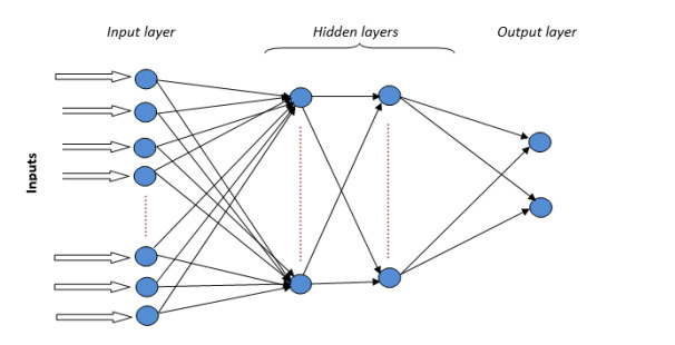
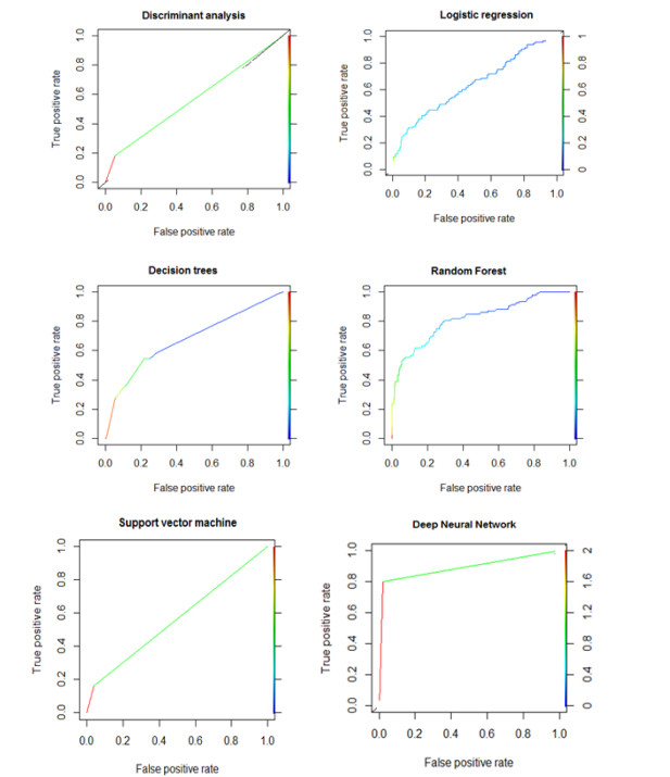
Credit scoring using machine learning and deep Learning-Based models

Sami Mestiri; Sami Mestiri

doi:10.3934/DSFE.2024009

Data Science in Finance and Economics

2024, Volume 4, Issue 2: 236-248. doi: 10.3934/DSFE.2024009

Previous Article Next Article

Research article Special Issues

Credit scoring using machine learning and deep Learning-Based models

Sami Mestiri ^{1,2
,
,}

1.
Faculty of Management and Economic Sciences of Mahdia, University of Monastir, Tunisia
2.
Sidi Messaoud Hiboun, Mahdia, Tunisia

Received: 23 December 2023 Revised: 15 March 2024 Accepted: 10 April 2024 Published: 07 May 2024
JEL Codes: C530, G210, G33

Credit scoring is a useful tool for assessing the capability of customers repayments. The purpose of this paper is to compare the predictive abilities of six credit scoring models: Linear Discriminant Analysis (LDA), Random Forests (RF), Logistic Regression (LR), Decision Trees (DT), Support Vector Machines (SVM) and Deep Neural Network (DNN). To compare these models, an empirical study was conducted using a sample of 688 observations and twelve variables. The performance of this model was analyzed using three measures: Accuracy rate, F1 score, and Area Under Curve (AUC). In summary, machine learning techniques exhibited greater accuracy in predicting loan defaults compared to other traditional statistical models.
- credit scoring,
- machine learning,
- artificial intelligence,
- model comparison,
- personal loan
Citation: Sami Mestiri. Credit scoring using machine learning and deep Learning-Based models[J]. Data Science in Finance and Economics, 2024, 4(2): 236-248. doi: 10.3934/DSFE.2024009

Related Papers:

Abstract

Credit scoring is a useful tool for assessing the capability of customers repayments. The purpose of this paper is to compare the predictive abilities of six credit scoring models: Linear Discriminant Analysis (LDA), Random Forests (RF), Logistic Regression (LR), Decision Trees (DT), Support Vector Machines (SVM) and Deep Neural Network (DNN). To compare these models, an empirical study was conducted using a sample of 688 observations and twelve variables. The performance of this model was analyzed using three measures: Accuracy rate, F1 score, and Area Under Curve (AUC). In summary, machine learning techniques exhibited greater accuracy in predicting loan defaults compared to other traditional statistical models.

References

[1]	Breiman L (2001) Random forests. Mach Learn 45: 5–32. https://doi.org/10.1023/A:1010933404324 doi: 10.1023/A:1010933404324
[2]	Deng L, Yu D (2014) Deep Learning: Methods and Applications. Found Trends Signal Proc 7: 197–387. http://dx.doi.org/10.1561/2000000039 doi: 10.1561/2000000039
[3]	Fuster A, Goldsmith Pinkham P, Ramadorai T, et al. (2022) Predictably unequal? The effects of machine learning on credit markets. J Financ 77: 5–47. https://doi.org/10.1111/jofi.12915 doi: 10.1111/jofi.12915
[4]	Giudici P, Hadji-Misheva B, Spelta A (2020) Network based credit risk models. Qual Eng 32: 199–211. https://doi.org/10.1080/08982112.2019.1655159 doi: 10.1080/08982112.2019.1655159
[5]	Le Cun Y, Bengio Y, Hinton GE (2015) Deep learning. Nature 521: 436–444. https://doi.org/10.1038/nature14539 doi: 10.1038/nature14539
[6]	Lyn T, David Edelman, Jonathan Crook (2002) Credit Scoring and its Applications. Mathematical Modeling and Computation. https://doi.org/10.1137/1.9780898718317 doi: 10.1137/1.9780898718317
[7]	Liu RL (2018) Machine learning approaches to predict default of credit card clients. Modern Econ 9: 18–28. https://doi.org/10.4236/me.2018.911115 doi: 10.4236/me.2018.911115
[8]	Lien CH, Yeh IC (2009) The Comparisons of Data Mining Techniques for the Predictive Accuracy of Probability of Default of Credit Card Clients. Expert Syst Appl 36: 2473–2480. https://doi.org/10.1016/j.eswa.2007.12.020 doi: 10.1016/j.eswa.2007.12.020
[9]	Mellisa K (2020) Credit Scoring Approaches guidelines. World Bank Group, Washington, DC, USA.
[10]	Mestiri S (2024) Financial Applications of Machine Learning Using R Software. SSRN Electronic J. https://dx.doi.org/10.2139/ssrn.4716425 doi: 10.2139/ssrn.4716425
[11]	Mestiri S, Farhat A (2021) Using Non-parametric Count Model for Credit Scoring. J Quant Econ 19: 39–49. https://doi.org/10.1007/s40953-020-00208-w doi: 10.1007/s40953-020-00208-w
[12]	Pepe MS (2000) Receiver operating characteristic methodology. J Am Stat Assoc 95: 308–311. https://doi.org/10.2307/2669554 doi: 10.2307/2669554
[13]	Giudici P (2001) Bayesian data mining, with application to credit scoring and benchmarking. Appl Stoch Models Bus Ind 17: 69–81. https://doi.org/10.1002/asmb.425 doi: 10.1002/asmb.425
[14]	Quinlan JR (1986) Induction of decision trees. Mach Learn 1: 81–106.
[15]	Tran K, Duong T, Ho Q (2016) Credit scoring model: A combination of genetic programming and deep learning, In: 2016 future technologies conference (ftc) IEEE, 145–149.
[16]	Schmidhuber J (2015) Deep learning in neural networks: An overview. Neural Networks 61: 85–117. https://doi.org/10.48550/arXiv.1404.7828 doi: 10.48550/arXiv.1404.7828
[17]	Stefan Lessmann, Bart Baesens, Hsin-Vonn Seow, et al. (2015) Benchmarking state-of-the-art classification algorithms for credit scoring: An update of research. Eur J Oper Res 247: 124–136. https://doi.org/10.1016/j.ejor.2015.05.030 doi: 10.1016/j.ejor.2015.05.030
[18]	Vapnik V (1998) The nature of statistical learning theory. New York: Springer.
[19]	Woo H, Sohn SY (2022) A credit scoring model based on the Myers–Briggs type indicator in online peer-to-peer lending. Financ Innov 8: 1–19. https://doi.org/10.1186/s40854-022-00347-4 doi: 10.1186/s40854-022-00347-4
[20]	Wang C, Han D, Liu Q, et al. (2018) A deep learning approach for credit scoring of peer-to-peer lending using attention mechanism LSTM. IEEE Access 7: 2161–2168. https://doi.org/10.1109/ACCESS.2018.2887138. doi: 10.1109/ACCESS.2018.2887138

Reader Comments

Your name:*

Email:*
© 2024 the Author(s), licensee AIMS Press. This is an open access article distributed under the terms of the Creative Commons Attribution License (http://creativecommons.org/licenses/by/4.0)