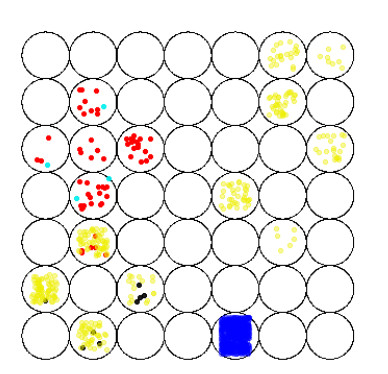
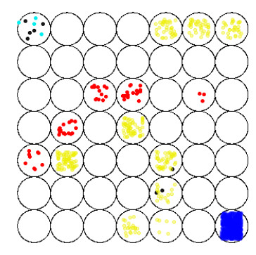
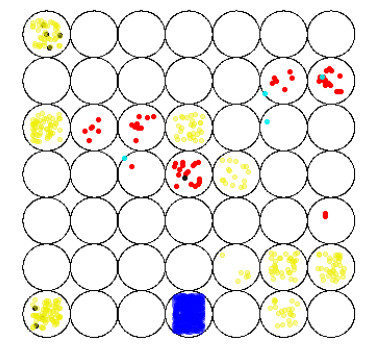
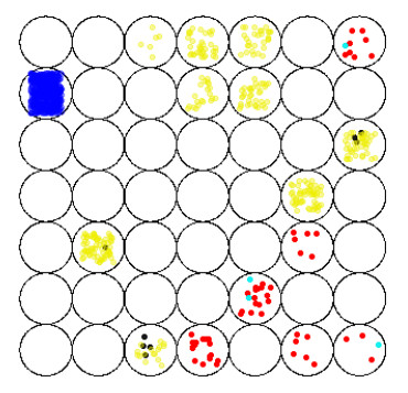
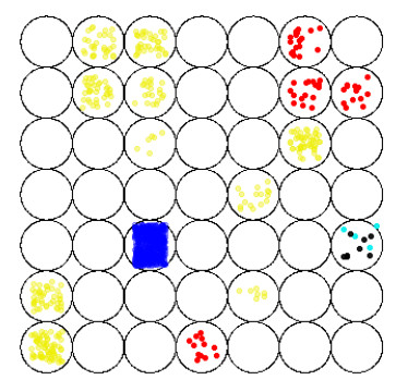
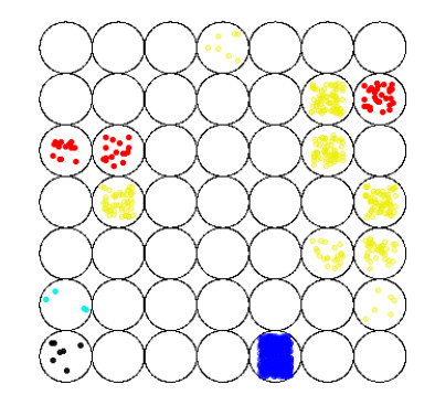
Bereavement exclusion (BE) is a criterion for excluding the diagnosis of major depressive disorder (MDD). Simplistically, this criterion states that an individual who reports MDD symptoms should not be diagnosed as suffering from this mental illness, if such an individual is grieving a sorrowful loss. BE was introduced in 1980 to avoid confusing MDD with normal grief, because several cognitive and physical symptoms of grief and depression can look similar. However, in 2013, BE was removed from the MDD diagnosis guidelines. Here, this controversial topic is computationally investigated. A virtual population is generated according to the Brazilian data of death rate and MDD prevalence and its five kinds of individuals are clustered by using a Kohonen's self-organizing map (SOM). In addition, by examining the current guidelines for diagnosing MDD from an analytical perspective, a slight modification is proposed. With this modification, an adequate clustering is achieved by the SOM neural network. Therefore, for mathematical consistency, unbalanced scores should be assigned to the items composing the MDD diagnostic criteria. With the proposed criteria, the co-occurrence of normal grief and MDD can also be satisfactorily clustered.
Citation: R. Loula, L. H. A. Monteiro. On the criteria for diagnosing depression in bereaved individuals: a self-organizing map approach[J]. Mathematical Biosciences and Engineering, 2022, 19(6): 5380-5392. doi: 10.3934/mbe.2022252
Bereavement exclusion (BE) is a criterion for excluding the diagnosis of major depressive disorder (MDD). Simplistically, this criterion states that an individual who reports MDD symptoms should not be diagnosed as suffering from this mental illness, if such an individual is grieving a sorrowful loss. BE was introduced in 1980 to avoid confusing MDD with normal grief, because several cognitive and physical symptoms of grief and depression can look similar. However, in 2013, BE was removed from the MDD diagnosis guidelines. Here, this controversial topic is computationally investigated. A virtual population is generated according to the Brazilian data of death rate and MDD prevalence and its five kinds of individuals are clustered by using a Kohonen's self-organizing map (SOM). In addition, by examining the current guidelines for diagnosing MDD from an analytical perspective, a slight modification is proposed. With this modification, an adequate clustering is achieved by the SOM neural network. Therefore, for mathematical consistency, unbalanced scores should be assigned to the items composing the MDD diagnostic criteria. With the proposed criteria, the co-occurrence of normal grief and MDD can also be satisfactorily clustered.

| [1] | J. Bowlby, Loss: sadness and depression, N. Y. Basic Books, 1980. |
| [2] | C. M. Parkes, H. G. Prigerson, Bereavement: studies of grief in adult life, Routledge, Philadelphia, 2013. |
| [3] |
A. Iglewicz, K. Seay, S. D. Zetumer, S. Zisook, The removal of the bereavement exclusion in the DSM-5: exploring the evidence, Curr. Psychiatry Rep., 15 (2013), 413. https://doi.org/10.1007/s11920-013-0413-0 doi: 10.1007/s11920-013-0413-0

|
| [4] |
E. G. Karam, C. C. Tabet, D. Alam, W. Shamseddeen, Y. Chatila, Z. Mneimneh, et al., Bereavement related and non-bereavement related depressions: a comparative field study, J. Affect. Disord., 112 (2009), 102–110. https://doi.org/10.1016/j.jad.2008.03.016 doi: 10.1016/j.jad.2008.03.016
|
| [5] |
G. Parker, S. McCraw, A. Paterson, Clinical features distinguishing grief from depressive episodes: a qualitative analysis, J. Affect. Disord., 176 (2015), 43–47. https://doi.org/10.1016/j.jad.2015.01.063 doi: 10.1016/j.jad.2015.01.063
|
| [6] |
K. Thieleman, J. Cacciatore, The DSM-5 and the bereavement exclusion: a call for critical evaluation, Soc. Work, 58 (2013), 277–280. https://doi.org/10.1093/sw/swt021 doi: 10.1093/sw/swt021
|
| [7] |
J. C. Wakefield, M. B. First, Validity of the bereavement exclusion to major depression: does the empirical evidence support the proposal to eliminate the exclusion in DSM-5?, World Psychiatry, 11 (2012), 3–10. https://doi.org/10.1016/j.wpsyc.2012.01.002 doi: 10.1016/j.wpsyc.2012.01.002
|
| [8] |
J. C. Wakefield, M. F. Schmitz, Symptom quality versus quantity in judging prognosis: using NESARC predictive validators to locate uncomplicated major depression on the number-of-symptoms severity continuum, J. Affect. Disord., 208 (2017), 325–329. https://doi.org/10.1016/j.jad.2016.09.015 doi: 10.1016/j.jad.2016.09.015
|
| [9] |
P. Zachar, M. B. First, K. S. Kendler, The bereavement exclusion debate in the DSM-5: a history, Clin. Psychol. Sci., 5 (2017), 890–906. https://doi.org/10.1177/2167702617711284 doi: 10.1177/2167702617711284
|
| [10] | American Psychiatric Association, Diagnostic and Statistical Manual of Mental Disorders (DSM-Ⅲ), 3rd edition, Washington, 1980. |
| [11] | American Psychiatric Association, Diagnostic and Statistical Manual of Mental Disorders (DSM-5), 5th edition, Washington, 2013. |
| [12] |
U. R. Acharya, S. L. Oh, Y. Hagiwara, J. H. Tan, H. Adeli, D. P. Subha, Automated EEG-based screening of depression using deep convolutional neural network, Comput. Methods Programs Biomed., 161 (2018), 103–113. https://doi.org/10.1016/j.cmpb.2018.04.012 doi: 10.1016/j.cmpb.2018.04.012
|
| [13] |
J. Gong, G. E. Simon, S. Liu, Machine learning discovery of longitudinal patterns of depression and suicidal ideation, PLoS One, 14 (2019), e0222665. https://doi.org/10.1371/journal.pone.0222665 doi: 10.1371/journal.pone.0222665
|
| [14] |
S. F. Lu, X. Shi, M. Li, J. A. Jiao, L. Feng, G. Wang, Semi-supervised random forest regression model based on co-training and grouping with information entropy for evaluation of depression symptoms severity, Math. Biosci. Eng., 18 (2021), 4586–4602. https://doi.org/10.3934/mbe.2021233 doi: 10.3934/mbe.2021233
|
| [15] |
M. L. Joshi, N. Kanoongo, Depression detection using emotional artificial intelligence and machine learning: a closer review, Mater. Today Proc., (2022), forthcoming. https://doi.org/10.1016/j.matpr.2022.01.467 doi: 10.1016/j.matpr.2022.01.467
|
| [16] |
N. V. Babu, E. G. M. Kanaga, Sentiment analysis in social media data for depression detection using artificial intelligence: a review, SN Comput. Sci., 3 (2022), 74. https://doi.org/10.1007/s42979-021-00958-1 doi: 10.1007/s42979-021-00958-1
|
| [17] | T. Kolenik, Methods in digital mental health: smartphone-based assessment and intervention for stress, anxiety, and depression, in Integrating Artificial Intelligence and IoT for Advanced Health Informatics (eds. C. Comito, A. Forestiero and E. Zumpano), Springer, (2022), 105–128. https://doi.org/10.1007/978-3-030-91181-2_7 |
| [18] |
K. Kaczmarek-Majer, G. Casalino, G. Castellano, O. Hryniewicz, M. Dominiak, Explaining smartphone-based acoustic data in bipolar disorder: semi-supervised fuzzy clustering and relative linguistic summaries, Inf. Sci., 588 (2022), 174–195. https://doi.org/10.1016/j.ins.2021.12.049 doi: 10.1016/j.ins.2021.12.049
|
| [19] |
T. Kohonen, The self-organizing map, Proc. IEEE, 78 (1990), 1464–1480. https://doi.org/10.1109/5.58325 doi: 10.1109/5.58325
|
| [20] |
T. Kohonen, Essentials of the self-organizing map, Neural Netwoks, 37 (2013), 52–65. https://doi.org/10.1016/j.neunet.2012.09.018 doi: 10.1016/j.neunet.2012.09.018
|
| [21] |
E. I. Fried, R. M. Nesse, Depression sum-scores don't add up: why analyzing specific depression symptoms is essential, BMC Med., 13 (2015), 72. https://doi.org/10.1186/s12916-015-0325-4 doi: 10.1186/s12916-015-0325-4
|
| [22] |
A. J. E. Kaiser, C. J. Funkhouser, V. A. Mittal, S. Walther, S. A. Shankman, Test-retest & familial concordance of MDD symptoms, Psychiatry Res., 292 (2020), 113313. https://doi.org/10.1016/j.psychres.2020.113313 doi: 10.1016/j.psychres.2020.113313
|
| [23] |
V. Lux, K. S. Kendler, Deconstructing major depression: a validation study of the DSM-Ⅳ symptomatic criteria, Psychol. Med., 40 (2010), 1679–1690. https://doi.org/10.1017/S0033291709992157 doi: 10.1017/S0033291709992157
|
| [24] |
M. Zimmerman, W. Ellison, D. Young, I. Chelminski, K. Dalrymple, How many different ways do patients meet the diagnostic criteria for major depressive disorder?, Compr. Psychiatry, 56 (2015), 29–34. https://doi.org/10.1016/j.comppsych.2014.09.007 doi: 10.1016/j.comppsych.2014.09.007
|
| [25] |
R. Loula, L. H. A. Monteiro, An individual-based model for predicting the prevalence of depression, Ecol. Complexity, 38 (2019), 168–172. https://doi.org/10.1016/j.ecocom.2019.03.003 doi: 10.1016/j.ecocom.2019.03.003
|
| [26] |
R. Loula, L. H. A. Monteiro, A game theory-based model for predicting depression due to frustration in competitive environments, Comput. Math. Method Med., 2020 (2020), 3573267. https://doi.org/10.1155/2020/3573267 doi: 10.1155/2020/3573267
|
| [27] |
R. Loula, L. H. A. Monteiro, Monoamine neurotransmitters and mood swings: a dynamical systems approach, Math. Biosci. Eng., 19 (2022), 4075–4083. https://doi.org/10.3934/mbe.2022187 doi: 10.3934/mbe.2022187
|
| [28] |
L. H. A. Monteiro, The grief map, Eur. Phys. J. Spec. Top., 223 (2014), 2897–2902. https://doi.org/10.1140/epjst/e2014-02302-0 doi: 10.1140/epjst/e2014-02302-0
|
| [29] |
Y. Kho, R. T. Kane, L. Priddis, J. Hudson, The nature of attachment relationships and grief responses in older adults: an attachment path model of grief, PLoS One, 10 (2015), e0133703. https://doi.org/10.1371/journal.pone.0133703 doi: 10.1371/journal.pone.0133703
|
| [30] |
M. Malgaroli, F. Maccallum, G. A. Bonanno, Machine yearning: how advances in computational methods lead to new insights about reactions to loss, Curr. Opin. Psychol., 43 (2022), 13–17. https://doi.org/10.1016/j.copsyc.2021.05.003 doi: 10.1016/j.copsyc.2021.05.003
|
| [31] | World Health Organization (WHO), Depression and other Common Mental Disorders: Global Health Estimates, Geneva, 2017. |
| [32] | Instituto Brasileiro de Geografia e Estatística (IBGE), População: Taxas Brutas de Mortalidade, IBGE, 2018. Available from: http://brasilemsintese.ibge.gov.br/populacao/taxas-brutas-de-mortalidade.html. |
| [33] |
C. Shannon, W. Weaver, N. Wiener, The mathematical theory of communication, Phys. Today, 3 (1950), 31. https://doi.org/10.1063/1.3067010 doi: 10.1063/1.3067010
|
| [34] | O. C. L. Haas, K. J. Burnham, Intelligent and Adaptive Systems in Medicine, CRC Press, Boca Raton, 2019. |
| [35] |
C. L. Wallace, S. P. Wladkowski, A. Gibson, P. White, Grief during the COVID-19 pandemic: considerations for palliative care providers, J. Pain Symptom Manage., 60 (2020), e70–e76. https://doi.org/10.1016/j.jpainsymman.2020.04.012 doi: 10.1016/j.jpainsymman.2020.04.012
|
| [36] |
J. P. Rogers, E. Chesney, D. Oliver, T. A. Pollak, P. McGuire, P. Fusar-Poli, et al., Psychiatric and neuropsychiatric presentations associated with severe coronavirus infections: a systematic review and meta-analysis with comparison to the COVID-19 pandemic, Lancet Psychiatry, 7 (2020), 611–627. https://doi.org/10.1016/S2215-0366(20)30203-0 doi: 10.1016/S2215-0366(20)30203-0
|
Figures(6) / Tables(1)

R. Loula, L. H. A. Monteiro. On the criteria for diagnosing depression in bereaved individuals: a self-organizing map approach[J]. Mathematical Biosciences and Engineering, 2022, 19(6): 5380-5392. doi: 10.3934/mbe.2022252


 DownLoad: