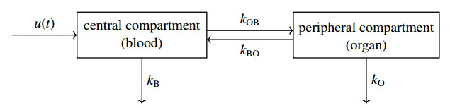
We consider a two-box model for the administration of a therapeutic substance and discuss two scenarios: First, the substance should have an optimal therapeutic concentration in the central compartment (typically blood) and be degraded in an organ, the peripheral compartment (e.g., the liver). In the other scenario, the concentration in the peripheral compartment should be optimized, with the blood serving only as a means of transport. In either case the corresponding optimal control problem is to determine a dosing schedule, i.e., how to administer the substance as a function $ u $ of time to the central compartment so that the concentration of the drug in the central or in the peripheral compartment remains as closely as possible at its optimal therapeutic level. We solve the optimal control problem for the central compartment explicitly by using the calculus of variations and the Laplace transform. We briefly discuss the effect of the approximation of the Dirac delta distribution by a bolus. The optimal control function $ u $ for the central compartment satisfies automatically the condition $ u\ge 0 $. But for the peripheral compartment one has to solve an optimal control problem with the non-linear constraint $ u\ge 0 $. This problem does not seem to be widely studied in the current literature in the context of pharmacokinetics. We discuss this question and propose two approximate solutions which are easy to compute. Finally we use Pontryagin's Minimum Principle to deduce the exact solution for the peripheral compartment.
Citation: Norbert Hungerbühler. Optimal control in pharmacokinetic drug administration[J]. Mathematical Biosciences and Engineering, 2022, 19(5): 5312-5328. doi: 10.3934/mbe.2022249
We consider a two-box model for the administration of a therapeutic substance and discuss two scenarios: First, the substance should have an optimal therapeutic concentration in the central compartment (typically blood) and be degraded in an organ, the peripheral compartment (e.g., the liver). In the other scenario, the concentration in the peripheral compartment should be optimized, with the blood serving only as a means of transport. In either case the corresponding optimal control problem is to determine a dosing schedule, i.e., how to administer the substance as a function $ u $ of time to the central compartment so that the concentration of the drug in the central or in the peripheral compartment remains as closely as possible at its optimal therapeutic level. We solve the optimal control problem for the central compartment explicitly by using the calculus of variations and the Laplace transform. We briefly discuss the effect of the approximation of the Dirac delta distribution by a bolus. The optimal control function $ u $ for the central compartment satisfies automatically the condition $ u\ge 0 $. But for the peripheral compartment one has to solve an optimal control problem with the non-linear constraint $ u\ge 0 $. This problem does not seem to be widely studied in the current literature in the context of pharmacokinetics. We discuss this question and propose two approximate solutions which are easy to compute. Finally we use Pontryagin's Minimum Principle to deduce the exact solution for the peripheral compartment.

| [1] |
Y. Cherruault, M. Guerret, Parameters identification and optimal control in pharmacokinetics, Acta Appl. Math., 1 (1983), 105–120. https://doi.org/10.1007/BF00046831 doi: 10.1007/BF00046831

|
| [2] | B. Some, Y. Cherruault, Optimization and optimal control of pharmacokinetics, Biomedicine & pharmacotherapy, 40 (1986), 183–187. |
| [3] |
F. Angaroni, A. Graudenzi, M. Rossignolo, D. Maspero, T. Calarco, R. Piazza, et al., An optimal control framework for the automated design of personalized cancer treatments, Front. Bioeng. Biotechnol., 2020. https://doi.org/10.3389/fbioe.2020.00523 doi: 10.3389/fbioe.2020.00523
|
| [4] |
M. Leszczyński, U. Ledzewicz, H. Schättler, Optimal control for a mathematical model for chemotherapy with pharmacometrics, Math. Model. Nat. Phenom., 15 (2020), 23. https://doi.org/10.1051/mmnp/2020008 doi: 10.1051/mmnp/2020008
|
| [5] |
I. Irurzun-Arana, A. Janda, S. Ardanza-Trevijano, I. F. Trocóniz, Optimal dynamic control approach in a multi-objective therapeutic scenario: Application to drug delivery in the treatment of prostate cancer, PLoS Comput. Biol., 14 (2018), e1006087. https://doi.org/10.1371/journal.pcbi.1006087 doi: 10.1371/journal.pcbi.1006087
|
| [6] |
F. Bachmann, G. Koch, M. Pfister, G. Szinnai, J. Schropp, Optidose: Computing the individualized optimal drug dosing regimen using optimal control, J. Optim. Theory Appl., 189 (2021), 46–65. https://doi.org/10.1007/s10957-021-01819-w doi: 10.1007/s10957-021-01819-w
|
| [7] |
P. Sopasakis, P. Patrinos, H. Sarimveis, Robust model predictive control for optimal continuous drug administration, Comput. Methods Programs Biomed., 116 (2014), 193–204. https://doi.org/10.1016/j.cmpb.2014.06.003 doi: 10.1016/j.cmpb.2014.06.003
|
| [8] |
S. Lucia, M. Schliemann, R. Findeisen, E. Bullinger, A set-based optimal control approach for pharmacokinetic/pharmacodynamic drug dosage design, IFAC-PapersOnLine, 49 (2016), 797–802. https://doi.org/10.1016/j.ifacol.2016.07.286 doi: 10.1016/j.ifacol.2016.07.286
|
| [9] | L. T. Aschepkov, D. V. Dolgy, T. Kim, R. P. Agarwal, Optimal Control, Springer, Cham, 2016. |
| [10] | H. P. Geering, Optimal Control with Engineering Applications, Springer, Berlin, 2007. |
| [11] | S. Lenhart, J. T. Workman, Optimal Control Applied to Biological Models, New York, 2007. https://doi.org/10.1201/9781420011418 |
| [12] | S. E. Rosenbaum, Basic Pharmacokinetics and Pharmacodynamics: An Integrated Textbook and Computer Simulations, Wiley, 2016. |
| [13] |
F. H. Clarke, Inequality constraints in the calculus of variations, Can. J. Math., 29 (1977), 528–540. https://doi.org/10.4153/CJM-1977-055-6 doi: 10.4153/CJM-1977-055-6
|
| [14] | F. A. Valentine, The problem of lagrange with differential inequalities as added side conditions, in Traces and Emergence of Nonlinear Programming, (2014), 313–357. https://doi.org/10.1007/978-3-0348-0439-4_16 |
Figures(9)

Norbert Hungerbühler. Optimal control in pharmacokinetic drug administration[J]. Mathematical Biosciences and Engineering, 2022, 19(5): 5312-5328. doi: 10.3934/mbe.2022249


 DownLoad: