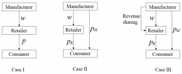
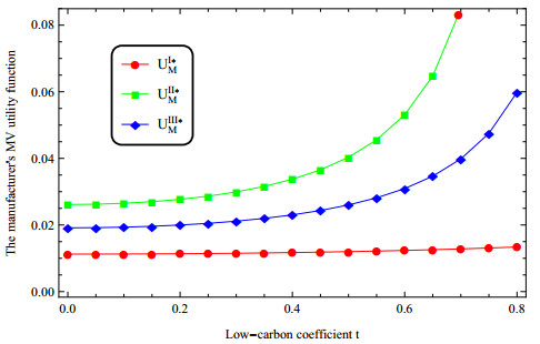
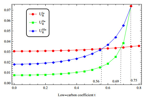
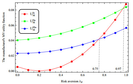
In a low-carbon supply chain (LCSC) constructed by a single manufacturer and a single retailer, three decision-making models are established by introducing channel preference attributes. That is, a single sales channel model, an online and offline dual channel model, and a dual channel model in which the manufacturer share revenue with her retailer. Using the mean variance (MV) method to characterize the risk aversion utility function of the manufacturer and the retailer, the following r are found. i) Consumers' preference for low-carbon products is conducive to raising the price of low-carbon products and the firms' profits. ii) The deepening of the retailer's risk aversion promotes the increase of the manufacturer's price, while the impact of the manufacturer's risk aversion has an opposite effects. Although the arbitrage behavior of the retailer can not be completely avoided in the risk aversion environment. However in a limited risk aversion environment, dual-channel development is conducive to increasing the profits of the manufacturer, but may harm the interests of the retailer. iii) Consumers' preference for online channel helps the manufacturer increase prices and profit. iv) The sharing of revenue by the manufacturer to the retailer is conducive to increasing the revenue of the retailer. Based on this, in order to improve corporate profits and promote long-term transactions, the manufacturer can carry out low-carbon promotion and implement a dual-channel strategy. The retailer can actively seek channel cooperation with the manufacturer.
Citation: Tao Li, Xin Xu, Kun Zhao, Chao Ma, Juan LG Guirao, Huatao Chen. Low-carbon strategies in dual-channel supply chain under risk aversion[J]. Mathematical Biosciences and Engineering, 2022, 19(5): 4765-4793. doi: 10.3934/mbe.2022223
In a low-carbon supply chain (LCSC) constructed by a single manufacturer and a single retailer, three decision-making models are established by introducing channel preference attributes. That is, a single sales channel model, an online and offline dual channel model, and a dual channel model in which the manufacturer share revenue with her retailer. Using the mean variance (MV) method to characterize the risk aversion utility function of the manufacturer and the retailer, the following r are found. i) Consumers' preference for low-carbon products is conducive to raising the price of low-carbon products and the firms' profits. ii) The deepening of the retailer's risk aversion promotes the increase of the manufacturer's price, while the impact of the manufacturer's risk aversion has an opposite effects. Although the arbitrage behavior of the retailer can not be completely avoided in the risk aversion environment. However in a limited risk aversion environment, dual-channel development is conducive to increasing the profits of the manufacturer, but may harm the interests of the retailer. iii) Consumers' preference for online channel helps the manufacturer increase prices and profit. iv) The sharing of revenue by the manufacturer to the retailer is conducive to increasing the revenue of the retailer. Based on this, in order to improve corporate profits and promote long-term transactions, the manufacturer can carry out low-carbon promotion and implement a dual-channel strategy. The retailer can actively seek channel cooperation with the manufacturer.

| [1] |
Q. Peng, C. Wang, L. Xu, Emission abatement and procurement strategies in a low-carbon supply chain with option contracts under stochastic demand, Comput. Ind. Eng., 144 (2020), 106502. https://doi.org/10.1016/j.cie.2020.106502 doi: 10.1016/j.cie.2020.106502

|
| [2] |
Y. Zhou, M. Bao, X. Chen, X. Xu, Co-op advertising and emission reduction cost sharing contracts and coordination in low-carbon supply chain based on fairness concerns, J. Cleaner Prod., 133 (2016), 402–413. https://doi.org/10.1016/j.jclepro.2016.05.097 doi: 10.1016/j.jclepro.2016.05.097
|
| [3] |
S. Shabir, N. A. AlBishri, Sustainable retailing performance of Zara during COVID-19 pandemic, Open J. Bus. Manage., 9 (2021), 1013–1029. https://doi.org/10.4236/ojbm.2021.93054 doi: 10.4236/ojbm.2021.93054
|
| [4] |
Y. Shen, J. Xie, T. Li, The risk-averse newsvendor game with competition on demand, J. Ind. Manage. Optimi., 12 (2016), 931–947. https://doi.org/10.3934/jimo.2016.12.931 doi: 10.3934/jimo.2016.12.931
|
| [5] |
S. Choi, A. Ruszczyński, A multi-product risk-averse newsvendor with exponential utility function, Eur. J. Oper. Res., 214 (2011), 78–84. https://doi.org/10.1016/j.ejor.2011.04.005 doi: 10.1016/j.ejor.2011.04.005
|
| [6] |
S. Choi, A. Ruszczyński, Y. Zhao, A multiproduct risk-averse newsvendor with law-invariant coherent measures of risk, Oper. Res., 59 (2011), 346–364. https://doi.org/10.1287/opre.1100.0896 doi: 10.1287/opre.1100.0896
|
| [7] |
S. A. Raza, S. M. Govindaluri, Pricing strategies in a dual-channel green supply chain with cannibalization and risk aversion, Oper. Res. Perspect., 6 (2019), 100118. https://doi.org/10.1016/j.orp.2019.100118 doi: 10.1016/j.orp.2019.100118
|
| [8] |
S. Du, L. Hu, L. Wang, Low-carbon supply policies and supply chain performance with carbon concerned demand, Ann. Oper. Res., 255 (2017), 569–590. https://doi.org/10.1007/s10479-015-1988-0 doi: 10.1007/s10479-015-1988-0
|
| [9] |
H. Peng, T. Pang, J. Cong, Coordination contracts for a supply chain with yield uncertainty and low-carbon preference, J. Cleaner Prod., 205 (2018), 291–302. https://doi.org/10.1016/j.jclepro.2018.09.038 doi: 10.1016/j.jclepro.2018.09.038
|
| [10] | Q. Han, Y. Wang, L. Shen, W. Dong, Decision and coordination of low-carbon E-commerce supply chain with government carbon subsidies and fairness concerns, Complexity, 2020 (2020). https://doi.org/10.1155/2020/1974942 |
| [11] |
J. Cong, T. Pang, H. Peng, Optimal strategies for capital constrained low-carbon supply chains under yield uncertainty, J. Cleaner Prod., 256 (2020), 120339. https://doi.org/10.1016/j.jclepro.2020.120339 doi: 10.1016/j.jclepro.2020.120339
|
| [12] |
H.Zou, J. Qin, B. Dai, Optimal pricing decisions for a low-carbon supply chain considering fairness concern under carbon quota policy, Int. J. Environ. Res. Public Health, 18 (2021), 556. https://doi.org/10.3390/ijerph18020556 doi: 10.3390/ijerph18020556
|
| [13] |
L. Xia, T. Guo, J. Qin, X. Yue, N. Zhu, Carbon emission reduction and pricing policies of a supply chain considering reciprocal preferences in cap-and-trade system, Ann. Oper. Res., 268 (2018), 149–175. https://doi.org/10.1007/s10479-017-2657-2 doi: 10.1007/s10479-017-2657-2
|
| [14] |
Y. Yu, S. Zhou, Y. Shi, Information sharing or not across the supply chain: The role of carbon emission reduction, Transp. Res. Part E: Logist. Transp. Rev., 137 (2020), 101915. https://doi.org/10.1016/j.tre.2020.101915 doi: 10.1016/j.tre.2020.101915
|
| [15] |
Y. Wu, R. Lu, J. Yang, F. Xu, Low-carbon decision-making model of online shopping supply chain considering the O2O model, J. Retailing Consum. Serv., 59 (2021), 102388. https://doi.org/10.1016/j.jretconser.2020.102388 doi: 10.1016/j.jretconser.2020.102388
|
| [16] |
S. K. Ghosh, M. R. Seikh, M. Chakrabortty, Analyzing a stochastic dual-channel supply chain under consumers' low carbon preferences and cap-and-trade regulation, Comput. Ind. Eng., 149 (2020), 106765. https://doi.org/10.1016/j.cie.2020.106765 doi: 10.1016/j.cie.2020.106765
|
| [17] | C. Che, Y. Chen, X. Zhang, Z. Zhang, The impact of different government subsidy methods on low-carbon emission reduction strategies in dual-channel supply chain, Complexity, 2021 (2021). https://doi.org/10.1155/2021/6668243 |
| [18] | G. Wang, X. Ai, H. Deng, Study on dual-channel revenue sharing coordination mechanisms based on the free riding, in 2009 6th International Conference on Service Systems and Service Management, (2009), 532–535. https://doi.org/10.1109/ICSSSM.2009.5174941 |
| [19] | Y. Liu, Z. Ding, Revenue sharing contract in dual channel supply chain in case of free riding, in Intelligent Decision Technologies, (2012), 459–469. https://doi.org/10.1007/978-3-642-29920-9_47 |
| [20] |
E. Cao, Coordination of dual-channel supply chains under demand disruptions management decisions, Int. J. Prod. Res., 52 (2014), 7114–7131. https://doi.org/10.1080/00207543.2014.938835 doi: 10.1080/00207543.2014.938835
|
| [21] |
L. Xu, C. Wang, J. Zhao, Decision and coordination in the dual-channel supply chain considering cap-and-trade regulation, J. Cleaner Prod., 197 (2018), 551–561. https://doi.org/10.1016/j.jclepro.2018.06.209 doi: 10.1016/j.jclepro.2018.06.209
|
| [22] |
C. H. Chiu, T. M. Choi, Supply chain risk analysis with mean-variance models: A technical review, Ann. Oper. Res., 240 (2016), 489–507. https://doi.org/10.1007/s10479-013-1386-4 doi: 10.1007/s10479-013-1386-4
|
| [23] |
W. Zhuo, L. Shao, H. Yang, Mean-variance analysis of option contracts in a two-echelon supply chain, Eur. J. Oper. Res., 271 (2018), 535–547. https://doi.org/10.1016/j.ejor.2018.05.033 doi: 10.1016/j.ejor.2018.05.033
|
| [24] |
T. M. Choi, X. Wen, X. Sun, S. H. Chung, The mean-variance approach for global supply chain risk analysis with air logistics in the blockchain technology era, Transp. Res. Part E: Logist. Transp. Rev., 127 (2019), 178–191. https://doi.org/10.1016/j.tre.2019.05.007 doi: 10.1016/j.tre.2019.05.007
|
| [25] |
X. Wen, T. Siqin, How do product quality uncertainties affect the sharing economy platforms with risk considerations? A mean-variance analysis, Int. J. Prod. Econ., 224 (2020), 107544. https://doi.org/10.1016/j.ijpe.2019.107544 doi: 10.1016/j.ijpe.2019.107544
|
| [26] | L. Qi, L. Liu, L. Jiang, Z. Wang, W. Zhao, Optimal operation strategies under a carbon cap-and-trade mechanism: A capital-constrained supply chain incorporating risk aversion, Math. Probl. Eng., 2020 (2020). https://doi.org/10.1155/2020/9515710 |
| [27] |
Q. Bai, F. Meng, Impact of risk aversion on two-echelon supply chain systems with carbon emission reduction constraints, J. Ind. Manage. Optim., 16 (2020), 1943–1965. https://doi.org/10.3934/jimo.2019037 doi: 10.3934/jimo.2019037
|
| [28] |
Z. Bao, Q. Wei, T. Zhou, X. Jiang, T. Watanabe, Predicting stock high price using forecast error with recurrent neural network, Appl. Math. Nonlinear Sci., 6 (2021), 283–292. https://doi.org/10.2478/amns.2021.2.00009 doi: 10.2478/amns.2021.2.00009
|
| [29] | Y. Zhang, J. Li, B. Xu, Designing buy-online-and-pick-up-in-store (BOPS) contract of dual-channel low-carbon supply chain considering consumers' low-carbon preference, Math. Probl. Eng., 2020 (2020). https://doi.org/10.1155/2020/7476019 |
| [30] |
X. Wang, M. Xue, L. Xing, Analysis of carbon emission reduction in a dual-channel supply chain with cap-and-trade regulation and low-carbon preference, Sustainability, 10 (2018), 580. https://doi.org/10.3390/su10030580 doi: 10.3390/su10030580
|
| [31] |
Q. Bai, J. Xu, S. S. Chauhan, Effects of sustainability investment and risk aversion on a two-stage supply chain coordination under a carbon tax policy, Comput. Ind. Eng., 142 (2020), 106324. https://doi.org/10.1016/j.cie.2020.106324 doi: 10.1016/j.cie.2020.106324
|
| [32] |
G. Xu, B. Dan, X. Zhang, C. Liu, Coordinating a dual-channel supply chain with risk-averse under a two-way revenue sharing contract, Int. J. Prod. Econ., 147 (2014), 171–179. https://doi.org/10.1016/j.ijpe.2013.09.012 doi: 10.1016/j.ijpe.2013.09.012
|
| [33] | G. Liu, T. Yang, Y. Wei, X. Zhang, Decisions on dual-channel supply chains under market fluctuations and dual-risk aversion, Discrete Dyn. Nat. Soc., 2020 (2020). https://doi.org/10.1155/2020/2612357 |
| [34] |
J. Y. Lee, S. Choi, Supply chain investment and contracting for carbon emissions reduction: A social planner's perspective, Int. J. Prod. Econ., 231 (2021), 107873. https://doi.org/10.1016/j.ijpe.2020.107873 doi: 10.1016/j.ijpe.2020.107873
|
| [35] |
Q. Li, B. Li, P. Chen, P. Hou, Dual-channel supply chain decisions under asymmetric information with a risk-averse retailer, Ann. Oper. Res., 257 (2017), 423–447. https://doi.org/10.1007/s10479-015-1852-2 doi: 10.1007/s10479-015-1852-2
|
| [36] | K. Matsui, When should a manufacturer set its direct price and wholesale price in dual-channel supply chains? Eur. J. Oper. Res., 258 (2017), 501–511. https://doi.org/10.1016/j.ejor.2016.08.048 |
| [37] |
P. Chen, R. Zhao, Y. Yan, C. Zhou, Promoting end-of-season product through online channel in an uncertain market, Eur. J. Oper. Res., 295 (2021), 935–948. https://doi.org/10.1016/j.ejor.2021.03.043 doi: 10.1016/j.ejor.2021.03.043
|
| [38] |
L. Sun, X. Jiao, X. Guo, Y. Yu, Pricing policies in dual distribution channels: The reference effect of official prices, Eur. J. Oper. Res., 296 (2022), 146–157. https://doi.org/10.1016/j.ejor.2021.03.040 doi: 10.1016/j.ejor.2021.03.040
|
| [39] |
G. Zhang, P. Cheng, H. Sun, Y. Shi, G. Zhang, A. Kadiane, Carbon reduction decisions under progressive carbon tax regulations: A new dual-channel supply chain network equilibrium model, Sustainable Prod. Consumption, 27 (2021), 1077–1092. https://doi.org/10.1016/j.spc.2021.02.029 doi: 10.1016/j.spc.2021.02.029
|
| [40] |
S. Choi, A loss-averse newsvendor with cap-and-trade carbon emissions regulation, Sustainability, 10 (2018), 2126. https://doi.org/10.3390/su10072126 doi: 10.3390/su10072126
|
| [41] |
S. Choi, K. Park, S. O. Shim, The optimal emission decisions of sustainable production with innovative baseline credit regulations, Sustainability, 11 (2019), 1635. https://doi.org/10.3390/su11061635 doi: 10.3390/su11061635
|
| [42] |
J. Liu, F. Huang, C. Ma, Coordination of VMI supply chain with replenishment tactic under risk aversion and sales effort, 4OR-Q. J. Oper. Res., 19 (2021), 389–414. https://doi.org/10.1007/s10288-020-00450-1 doi: 10.1007/s10288-020-00450-1
|
Figures(11) / Tables(2)

Tao Li, Xin Xu, Kun Zhao, Chao Ma, Juan LG Guirao, Huatao Chen. Low-carbon strategies in dual-channel supply chain under risk aversion[J]. Mathematical Biosciences and Engineering, 2022, 19(5): 4765-4793. doi: 10.3934/mbe.2022223


 DownLoad: