Frequency of hereditary hemochromatosis gene mutations and their effects on iron overload among beta thalassemia patients of Chennai residents

Bhuvana Selvaraj; Sangeetha Soundararajan; Shettu Narayanasamy; Ganesan Subramanian; Senthil Kumar Ramanathan; Bhuvana Selvaraj; Sangeetha Soundararajan; Shettu Narayanasamy; Ganesan Subramanian; Senthil Kumar Ramanathan

doi:10.3934/molsci.2021018

AIMS Molecular Science

2021, Volume 8, Issue 4: 233-247. doi: 10.3934/molsci.2021018

Previous Article Next Article

Research article

Frequency of hereditary hemochromatosis gene mutations and their effects on iron overload among beta thalassemia patients of Chennai residents

1.
Department of Molecular Biology, Dr. Ganesan's Hitech Diagnostic centre, Chennai, Tamil Nadu, India
2.
PG and Research Department of Zoology, Pachaiyappa's College, University of Madras, Chennai, Tamil Nadu, India
3.
Department of Pathology, Dr. Ganesan's Hitech Diagnostic centre, Chennai, Tamil Nadu, India
4.
Department of Molecular Biology, Dr. Ganesan's Hitech Diagnostic centre, Chennai, Tamil Nadu, India

Received: 09 September 2021 Accepted: 09 November 2021 Published: 12 November 2021

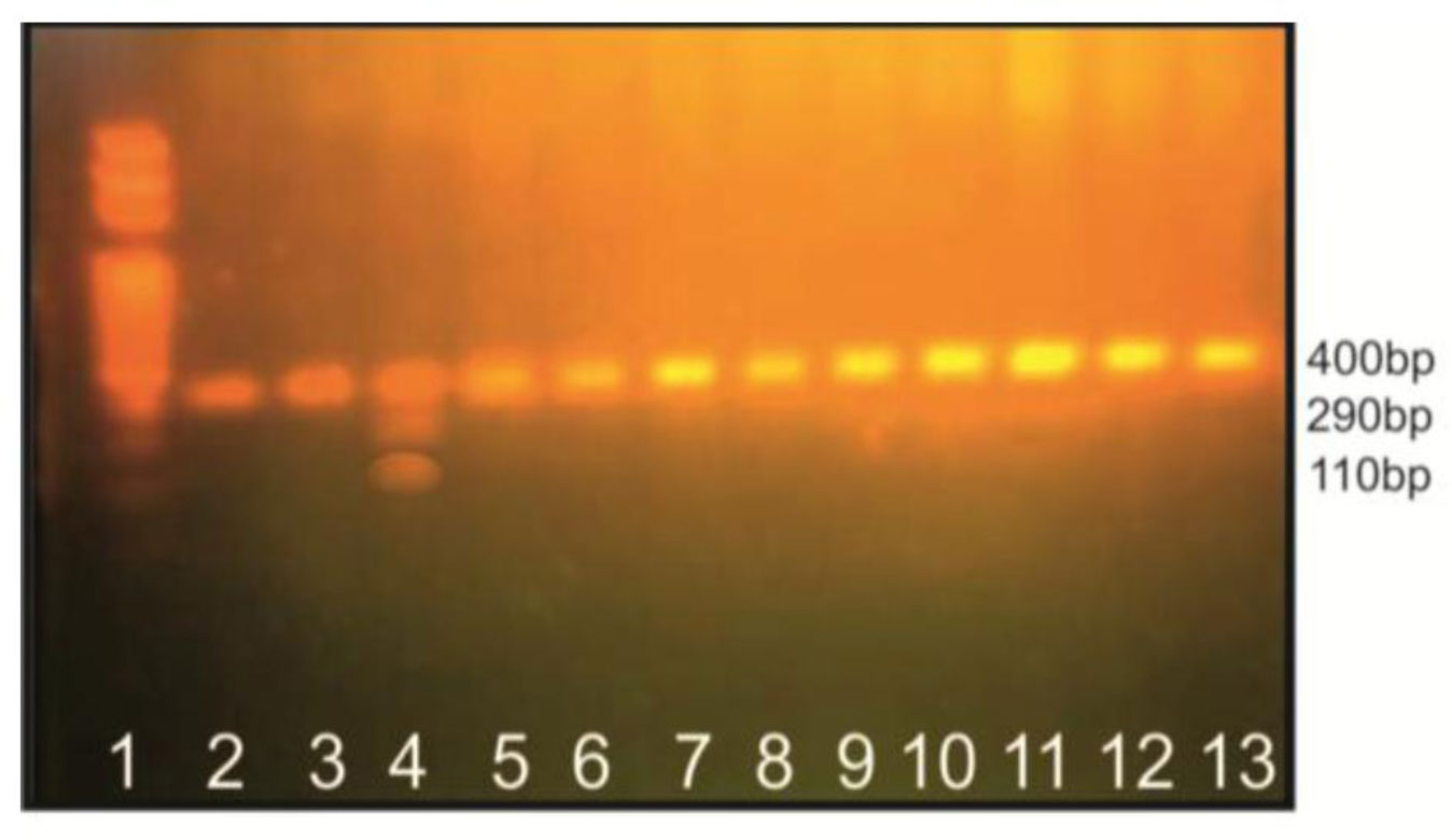
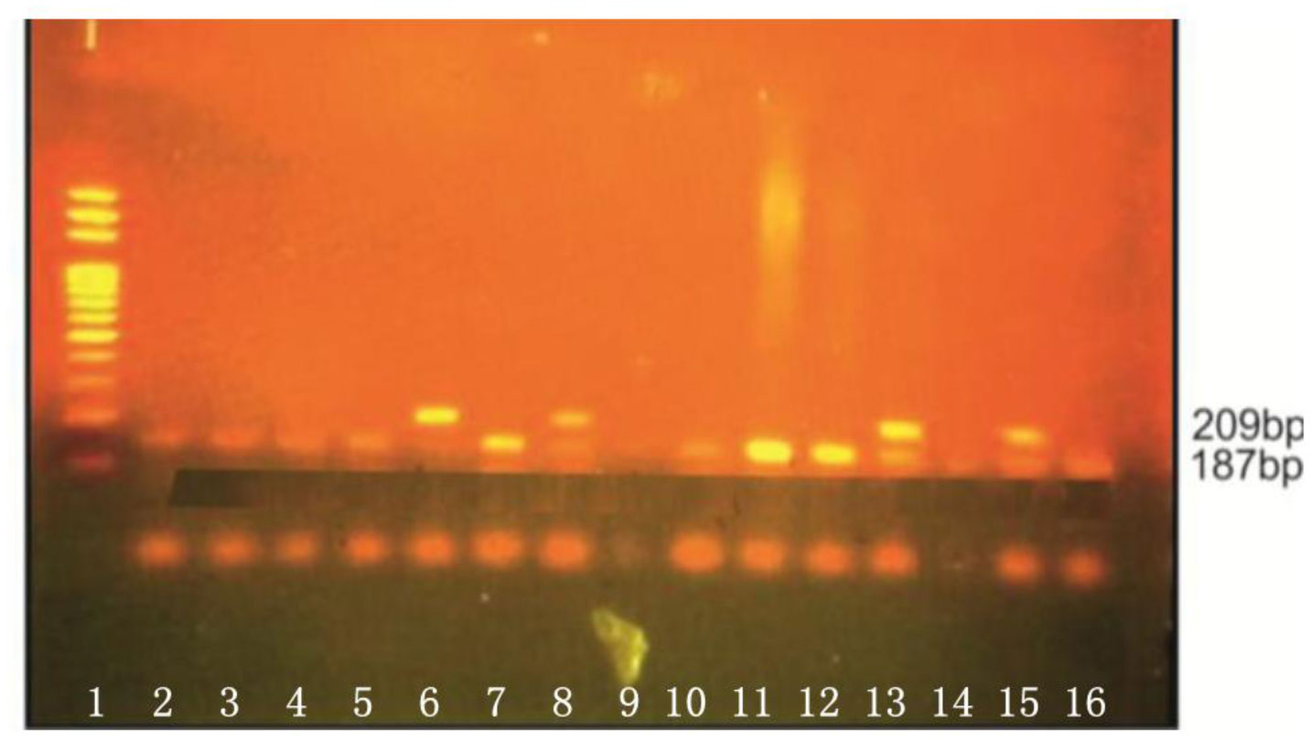
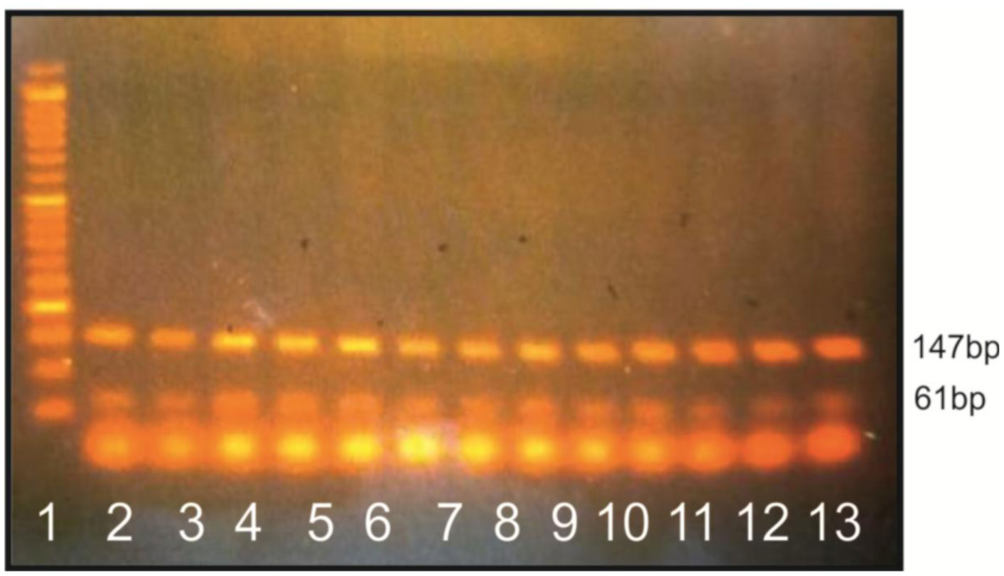
Hereditary Hemochromatosis (HH) is an autosomal recessive disorder of iron metabolism associated with HFE gene mutations, characterized by increased iron absorption and accumulation leading to multi-organ damage caused by iron overload toxicity. Beta thalassemia is caused by a mutation in the human beta globin gene. Imbalanced production of globin chain results in beta thalassemia, where the unpaired alpha chains precipitates in red cell precursors leading to ineffective erythropoiesis and reduced RBC survival. Both HH and beta thalassemia condition results in rapid accumulation of iron lead to iron overload in tissues and organs. The study aims to analyze the frequency of HFE variants among beta thalassemia cases and their effect on iron overload. The frequency of three HFE variants C282Y, H63D, S65C was analyzed by PCR RFLP method among Beta Thalassemia Trait (BTT) (n = 203), Beta Thalassemia Major (BTM) (n = 19) and age and sex-matched control samples (n = 200). The present study furnished allele frequency of H63D variant in BTT, BTM and controls 8.13, 15.8 and 6% respectively. Ten out of 33 heterozygous H63D variants exhibited iron overload with higher ferritin levels indicating HFE variant might aggravate the absorption of iron. The C282Y variant was present in heterozygous state in 1 case among beta thalassemia carriers. The C282Y variant was absent among BTM and control cases. S65C HFE variant was absent in the present study. Iron overload was completely absent in the control cases among all three HFE genotypes. Hence it is inferred from the present investigation, analysis of HFE genes and iron status will remarkably help to reason out the probable reason behind the iron status and support in proper management of beta thalassemia cases.

Keywords:

Citation: Bhuvana Selvaraj, Sangeetha Soundararajan, Shettu Narayanasamy, Ganesan Subramanian, Senthil Kumar Ramanathan. Frequency of hereditary hemochromatosis gene mutations and their effects on iron overload among beta thalassemia patients of Chennai residents[J]. AIMS Molecular Science, 2021, 8(4): 233-247. doi: 10.3934/molsci.2021018

Related Papers:

[1]	Dojin Kim, Patcharee Wongsason, Jongkyum Kwon . Type 2 degenerate modified poly-Bernoulli polynomials arising from the degenerate poly-exponential functions. AIMS Mathematics, 2022, 7(6): 9716-9730. doi: 10.3934/math.2022541
[2]	Taekyun Kim, Dae San Kim, Dmitry V. Dolgy, Hye Kyung Kim, Hyunseok Lee . A new approach to Bell and poly-Bell numbers and polynomials. AIMS Mathematics, 2022, 7(3): 4004-4016. doi: 10.3934/math.2022221
[3]	Jongkyum Kwon, Patcharee Wongsason, Yunjae Kim, Dojin Kim . Representations of modified type 2 degenerate poly-Bernoulli polynomials. AIMS Mathematics, 2022, 7(6): 11443-11463. doi: 10.3934/math.2022638
[4]	Sang Jo Yun, Jin-Woo Park . On a generation of degenerate Daehee polynomials. AIMS Mathematics, 2025, 10(5): 12286-12298. doi: 10.3934/math.2025556
[5]	Taekyun Kim, Hye Kyung Kim, Dae San Kim . Some identities on degenerate hyperbolic functions arising from $ p $-adic integrals on $ \mathbb{Z}_p $. AIMS Mathematics, 2023, 8(11): 25443-25453. doi: 10.3934/math.20231298
[6]	Taekyun Kim, Dae San Kim, Hye Kyung Kim . Some identities involving degenerate Stirling numbers arising from normal ordering. AIMS Mathematics, 2022, 7(9): 17357-17368. doi: 10.3934/math.2022956
[7]	Taekyun Kim, Dae San Kim, Hyunseok Lee, Lee-Chae Jang . A note on degenerate derangement polynomials and numbers. AIMS Mathematics, 2021, 6(6): 6469-6481. doi: 10.3934/math.2021380
[8]	Hye Kyung Kim, Dmitry V. Dolgy . Degenerate Catalan-Daehee numbers and polynomials of order $ r $ arising from degenerate umbral calculus. AIMS Mathematics, 2022, 7(3): 3845-3865. doi: 10.3934/math.2022213
[9]	Taekyun Kim, Dae San Kim, Jin-Woo Park . Degenerate $ r $-truncated Stirling numbers. AIMS Mathematics, 2023, 8(11): 25957-25965. doi: 10.3934/math.20231322
[10]	Jung Yoog Kang, Cheon Seoung Ryoo . The forms of $ (q, h) $-difference equation and the roots structure of their solutions with degenerate quantum Genocchi polynomials. AIMS Mathematics, 2024, 9(11): 29645-29661. doi: 10.3934/math.20241436

Abstract

Abbreviations

BTH:

Beta Thalassemia Homozygous;

BTM:

Beta Thalassemia Major;

BTT:

Beta Thalassemia Trait;

HBB:

Hemoglobin Subunit Beta gene;

HH:

Hereditary Hemochromatosis;

SNPs:

Single Nucleotide Polymorphism;

WT:

Wild type allele

1. Introduction

In ^[1,2], Carlitz initiated study of the degenerate Bernoulli and Euler polynomials and obtained some arithmetic and combinatorial results on them. In recent years, many mathematicians have drawn their attention to various degenerate versions of some old and new polynomials and numbers, namely some degenerate versions of Bernoulli numbers and polynomials of the second kind, Changhee numbers of the second kind, Daehee numbers of the second kind, Bernstein polynomials, central Bell numbers and polynomials, central factorial numbers of the second kind, Cauchy numbers, Eulerian numbers and polynomials, Fubini polynomials, Stirling numbers of the first kind, Stirling polynomials of the second kind, central complete Bell polynomials, Bell numbers and polynomials, type 2 Bernoulli numbers and polynomials, type 2 Bernoulli polynomials of the second kind, poly-Bernoulli numbers and polynomials, poly-Cauchy polynomials, and of Frobenius-Euler polynomials, to name a few ^{[3,14,16,17,18]} and the references therein. They have studied those polynomials and numbers with their interest not only in combinatorial and arithmetic properties but also in differential equations and certain symmetric identities ^[4,5] and references therein, and found many interesting results related to them ^{[12,19,20,21,22,23,24,25,26,27,28]}. It is remarkable that studying degenerate versions is not only limited to polynomials but also extended to transcendental functions.

The Bernoulli polynomials of the second are defined by as follows (see ^[9,13])

$\begin{align} \frac{z}{\log(1+z)}(1+z)^x = \sum\limits_{q = 0}^{\infty}b_q(x)\frac{z^q}{q!}. \end{align}$

(1.1)

When $x = 0$ , $b_q(0) = b_q$ are called the Bernoulli numbers of the second kind.

The degenerate exponential function $e_{\lambda}^{x}(z)$ is defined by (see ^{[6,7,8,9,10,11,12,13,14,15,16,17,18,19]})

$\begin{align} e_{\lambda}^{x}(z) = (1+\lambda z)^{\frac{x}{\lambda}}, \; \; e_{\lambda}(z) = (1+\lambda z)^{\frac{1}{\lambda}}, \; \lambda\in \mathbb{C}\backslash \{0\}. \end{align}$

(1.2)

We note that

$\begin{align} e_{\lambda}^{x}(z) = \sum\limits_{q = 0}^{\infty}(x)_{q, \lambda}\frac{z^q}{q!}, {\rm{(see \; [4, 21])}}, \end{align}$

(1.3)

where $(x)_{q, \lambda} = x(x-\lambda)\cdots(x-(q-1)\lambda), (q\geq1)$ , $(x)_{0, \lambda} = 1$ .

Note that

$\lim\limits_{\lambda\rightarrow 0}e_{\lambda}^{x}(z) = \sum\limits_{q = 0}^{\infty}x^q\frac{z^q}{q!} = e^{xz}.$

The degenerate Bernoulli polynomials which are defined by Carlitz's as follows (see ^[1,2])

$\begin{align} \frac{z}{e_{\lambda}(z)-1}e_{\lambda}^{x}(z) = \frac{z}{(1+\lambda z)^{\frac{1}{\lambda}}-1}(1+\lambda z)^{\frac{x}{\lambda}} = \sum\limits_{q = 0}^{\infty}\beta_{q}(x;\lambda)\frac{z^q}{q!}. \end{align}$

(1.4)

At the point $x = 0$ , $\beta_{q}(\lambda) = \beta_{q}(0;\lambda)$ are called the degenerate Bernoulli numbers.

Note that

$\lim\limits_{\lambda \longrightarrow 0}\beta_{q}(x;\lambda) = B_{q}(x).$

The polylogarithm function is defined by

$\begin{align} {\rm Li}_{k}(x) = \sum\limits_{q = 1}^{\infty}\frac{x^q}{q^k}\; \; \; (k\in\mathbb Z, \; \mid x\mid < 1), {\rm{(see \; [7])}}. \end{align}$

(1.5)

Note that

$\begin{align} {\rm Li}_{1}(x) = \sum\limits_{q = 1}^{\infty}\frac{x^q}{q} = -\log(1-x). \end{align}$

(1.6)

The poly-Bernoulli polynomials of the second are defined by (see ^[13])

$\begin{align} \frac{{\rm Li}_{k}(1-e^{-z})}{\log(1+z)}(1+z)^{x} = \sum\limits_{q = 0}^{\infty}b_{q}^{(k)}(x)\frac{z^q}{q!}. \end{align}$

(1.7)

In the case when $x = 0$ , $b_{q}^{(k)} = b_{q}^{(k)}(0)$ are called the poly-Bernoulli numbers of the second kind.

The modified degenerate polyexponential function is defined by (see ^[14])

$\begin{align} {\rm Ei}_{k, \lambda}(x) = \sum\limits_{q = 1}^{\infty}\frac{(1)_{q, \lambda}}{(q-1)!q^k}x^q. \end{align}$

(1.8)

It is noteworthy to mention that

${\rm Ei}_{1, \lambda}(x) = \sum\limits_{q = 1}^{\infty}\frac{(1)_{q, \lambda}}{q!}x^q = e_{\lambda}(x)-1.$

The degenerate poly-Genocchi polynomials which are defined by Kim et al. as follows (see ^[14])

$\begin{align} \frac{2{\rm Ei}_{k, \lambda}\left(\log_{\lambda}(1+z)\right)}{e_{\lambda}(z)+1}e_{\lambda}^{x}(z) = \sum\limits_{q = 0}^{\infty}G_{q, \lambda}^{(k)}(x)\frac{z^q}{q!}\; \; \; (k\in\mathbb Z). \end{align}$

(1.9)

When $x = 0$ , $G_{q, \lambda}^{(k)} = G_{q, \lambda}^{(k)}(0)$ are called the degenerate poly-Genocchi numbers.

For $\lambda\in\mathbb R$ , Kim-Kim defined the degenerate version of the logarithm function, denoted by $\log_{\lambda}(1+t)$ as follows (see ^[11])

$\begin{align} \log_{\lambda}(1+z) = \sum\limits_{q = 1}^{\infty}\lambda^{\lambda-1}(1)_{q, 1/\lambda}\frac{z^q}{q!}, \end{align}$

(1.10)

being the inverse of the degenerate version of the exponential function $e_{\lambda}(z)$ as has been shown below

$e_{\lambda}(\log_{\lambda}(z)) = \log_{\lambda}(e_{\lambda}(z)) = z.$

It is noteworthy to mention that

$\lim\limits_{\lambda\rightarrow 0}\log_{\lambda}(1+z) = \sum\limits_{q = 1}^{\infty}(-1)^{q-1}\frac{z^q}{q!} = \log(1+z).$

The degenerate Daehee polynomials are defined by (see ^[15])

$\begin{align} \frac{\log_{\lambda}(1+z)}{z}(1+z)^{x} = \sum\limits_{q = 0}^{\infty}D_{q, \lambda}(x)\frac{z^q}{q!}. \end{align}$

(1.11)

In the case when $x = 0$ , $D_{q, \lambda} = D_{q, \lambda}(0)$ denotes the degenerate Daehee numbers.

The degenerate Bernoulli polynomials of the second kind which are defined by Kim et al. as follows (see ^[9])

$\begin{align} \frac{z}{\log_{\lambda}(1+z)}(1+z)^{x} = \sum\limits_{q = 0}^{\infty}b_{q, \lambda}(x)\frac{z^q}{q!}. \end{align}$

(1.12)

When $x = 0$ , $b_{q, \lambda} = b_{q, \lambda}(0)$ are called the degenerate Bernoulli numbers of the second kind.

Note here that $\lim_{\lambda \rightarrow 0}b_{q, \lambda}(x) = b_q(x), (q\geq 0)$ .

The degenerate Stirling numbers of the first kind are defined by

$\begin{align} \frac{1}{k!}(\log_{\lambda}(1+z))^k = \sum\limits_{q = k}^{\infty}S_{1, \lambda}(q, k)\frac{z^q}{q!}\; \; (k\geq 0), \rm{(see \; [11, 12])}. \end{align}$

(1.13)

It is noticed that

$\lim\limits_{\lambda\rightarrow 0}S_{1, \lambda}(q, k) = S_1(q, k),$

are the Stirling numbers of the first kind presented by

$\frac{1}{k!}(\log(1+z))^k = \sum\limits_{q = k}^{\infty}S_{1}(q, k)\frac{z^q}{q!}\; \; (k\geq 0), {\rm{(see \; [7, 17])}}.$

The degenerate Stirling numbers of the second kind are defined by (see ^[8])

$\begin{align} \frac{1}{k!}(e_{\lambda}(z)-1)^k = \sum\limits_{q = k}^{\infty}S_{2, \lambda}(q, k)\frac{z^q}{q!}\; \; (k\geq 0). \end{align}$

(1.14)

It is clear that

$\lim\limits_{\lambda\rightarrow 0}S_{2, \lambda}(q, k) = S_2(q, k),$

are the Stirling numbers of the second kind specified by

$\frac{1}{k!}(e^z-1)^k = \sum\limits_{q = k}^{\infty}S_{2}(q, k)\frac{z^q}{q!}\; \; (k\geq 0), {\rm{(see \; [1-28])}}.$

Motivated by the works of Kim et al. ^[11,14], in this paper, we study the type 2 degenerate poly-Bernoulli polynomials of the second kind arising from modified degenerate polyexponential function and obtain some related identities and explicit expressions. Also, we establish the type 2 degenerate unipoly-Bernoulli polynomials of the second kind attached to an arithmetic function by using modified degenerate polyexponential function and discuss some properties of them.

2. Type 2 degenerate poly-Bernoulli polynomials of the second kind

Here, the type 2 degenerate poly-Bernoulli polynomials of the second kind are defined by using the modified degenerate polyexponential function which is called the degenerate poly-Bernoulli polynomials of the second kind as

$\begin{align} \frac{{\rm Ei}_{k, \lambda}\left(\log_{\lambda}(1+z)\right)}{\log_{\lambda}(1+z)}(1+z)^{x} = \sum\limits_{j = 0}^{\infty}Pb_{j, \lambda}^{(k)}(x)\frac{z^j}{j!}, (k\in\mathbb Z). \end{align}$

(2.1)

When $x = 0$ , $Pb_{j, \lambda}^{(k)} = Pb_{j, \lambda}^{(k)}(0)$ are called the type 2 degenerate poly-Bernoulli numbers of the second kind.

Note that

$\lim\limits_{\lambda\rightarrow 0}\frac{{\rm Ei}_{k, \lambda}\left(\log_{\lambda}(1+z)\right)}{\log_{\lambda}(1+z)}(1+z)^{x} = \sum\limits_{j = 0}^{\infty}\lim\limits_{\lambda\rightarrow 0}Pb_{j, \lambda}^{(k)}(x)\frac{z^j}{j!}$

$\begin{align} = \frac{{\rm Ei}_{k}\left(\log(1+z)\right)}{\log(1+z)}(1+z)^{x} = \sum\limits_{j = 0}^{\infty}Pb_{j}^{(k)}(x)\frac{z^j}{j!}, (k\in\mathbb Z), \end{align}$

(2.2)

where $Pb_{j}^{(k)}(x)$ are called the type 2 poly-Bernoulli polynomials of the second kind (see ^[9]).

First, we note that

${\rm Ei}_{k, \lambda}\left(\log_{\lambda}(1+z)\right) = \sum\limits_{q = 1}^{\infty}\frac{(1)_{q, \lambda}(\log_{\lambda}(1+z))^q}{(q-1)!q^k}$

$= \sum\limits_{q = 0}^{\infty}\frac{(1)_{q+1, \lambda}(\log_{\lambda}(1+z))^{q+1}}{(q+1)^kq!}$

$= \sum\limits_{q = 0}^{\infty}\frac{(1)_{q+1, \lambda}}{(q+1)^{k-1}}\frac{1}{(q+1)!}(\log_{\lambda}(1+z))^{q+1}$

$\begin{align} = \sum\limits_{q = 0}^{\infty}\frac{(1)_{q+1, \lambda}}{(q+1)^{k-1}}\sum\limits_{r = q+1}^{\infty}S_{1, \lambda}(r, q+1)\frac{z^r}{r!}. \end{align}$

(2.3)

By making use of (2.1) and (2.3), we see that

$\frac{z}{\log_{\lambda}(1+z)}(1+z)^{x}{\rm Ei}_{k, \lambda}\left(\log_{\lambda}(1+z)\right) \quad$

$= \frac{z}{\log_{\lambda}(1+z)}(1+z)^{x}\sum\limits_{q = 0}^{\infty}\frac{(1)_{q+1, \lambda}}{(q+1)^{k-1}} \sum\limits_{r = q}^{\infty}\frac{S_{1, \lambda}(r+1, q+1)}{r+1}\frac{z^r}{r!}$

$= \sum\limits_{j = 0}^{\infty}b_{j, \lambda}(x)\frac{z^j}{j!}\sum\limits_{q = 0}^{\infty}\frac{(1)_{q+1, \lambda}}{(q+1)^{k-1}}\sum\limits_{r = q}^{\infty} \frac{S_{1, \lambda}(r+1, q+1)}{r+1}\frac{z^r}{r!}$

$\begin{align} = \sum\limits_{j = 0}^{\infty}\left(\sum\limits_{r = 0}^{j}\binom{j}{r}\sum\limits_{q = 0}^{r}\frac{(1)_{q+1, \lambda}}{(q+1)^{k-1}}\frac{S_{1, \lambda}(r+1, q+1)}{r+1}b_{j-r, \lambda}(x)\right)\frac{z^j}{j!}. \end{align}$

(2.4)

Therefore, by (2.3) and (2.4), we obtain the following theorem.

Theorem 2.1. For $k\in\mathbb Z$ and $j\geq 0$ , we have

$Pb_{j, \lambda}^{(k)}(x) = \sum\limits_{r = 0}^{j}\binom{j}{r}\sum\limits_{q = 0}^{r}\frac{(1)_{q+1, \lambda}}{(q+1)^{k-1}}\frac{S_{1, \lambda}(r+1, q+1)}{r+1} b_{j-r, \lambda}(x).$

Corollary 2.1. Putting $k = 1$ in Theorem 2.1 yields

$Pb_{j, \lambda}(x) = \sum\limits_{r = 0}^{j}\binom{j}{r}\sum\limits_{q = 0}^{r}\frac{(1)_{q+1, \lambda}S_{1, \lambda}(r+1, q+1)}{r+1}b_{j-r, \lambda}(x).$

Let $1\leq k\in\mathbb{Z}$ . For $s\in\mathbb C$ , the function $\chi_{k, \lambda}(s)$ is given as

$\begin{align} \chi_{k, \lambda}(s) = \frac{1}{\Gamma (s)}\int_{0}^{\infty}\frac{z^{s-1}}{\log_{\lambda}(1+z)}{\rm Ei}_{k, \lambda}\left(\log_{\lambda}(1+z)\right)dz. \end{align}$

(2.5)

From Eq (2.5), we have

$\chi_{k, \lambda}(s) = \frac{1}{\Gamma (s)}\int_{0}^{\infty}\frac{z^{s-1}}{\log_{\lambda}(1+z)}{\rm Ei}_{k, \lambda}\left(\log_{\lambda}(1+z)\right)dz$

$= \frac{1}{\Gamma (s)}\int_{0}^{1}\frac{z^{s-1}}{\log_{\lambda}(1+z)}{\rm Ei}_{k, \lambda}\left(\log_{\lambda}(1+z)\right)dz$

$\begin{align} +\frac{1}{\Gamma (s)}\int_{1}^{\infty}\frac{z^{s-1}}{\log_{\lambda}(1+z)}{\rm Ei}_{k, \lambda}\left(\log_{\lambda}(1+z)\right)dz. \end{align}$

(2.6)

For any $s\in\mathbb C$ , the second integral is absolutely convergent and thus, the second term on the r.h.s. vanishes at non-positive integers. That is,

$\begin{align} \lim\limits_{s\rightarrow -m}\left|\frac{1}{\Gamma (s)}\int_{1}^{\infty}\frac{z^{s-1}}{\log_{\lambda}(1+z)}{\rm Ei}_{k, \lambda}\left(\log_{\lambda}(1+z)\right)dz\right|\leq\frac{1}{\Gamma(-m)}M = 0. \end{align}$

(2.7)

On the other hand, the first integral in Eq (2.7), for $\Re(s) > 0$ can be written as

$\frac{1}{\Gamma (s)}\sum\limits_{r = 0}^{\infty}\frac{Pb_{r, \lambda}^{(k)}}{r!}\frac{1}{s+r},$

which defines an entire function of $s$ . Thus, we may include that $\chi_{k, \lambda}(s)$ can be continued to an entire function of $s$ .

Further, from (2.6) and (2.7), we obtain

$\chi_{k, \lambda}(-m) = \lim\limits_{s\rightarrow -m}\frac{1}{\Gamma (s)}\int_{0}^{1}\frac{z^{s-1}}{\log_{\lambda}(1+z)}{\rm Ei}_{k, \lambda}\left(\log_{\lambda}(1+z)\right)dz$

$= \lim\limits_{s\rightarrow -m}\frac{1}{\Gamma (s)}\int_{0}^{1}z^{s-1}\sum\limits_{r = 0}^{\infty}\frac{Pb_{r, \lambda}^{(k)}z^r}{r!}dz = \lim\limits_{s\rightarrow -m}\frac{1}{\Gamma (s)}\sum\limits_{r = 0}^{\infty}\frac{Pb_{r, \lambda}^{(k)}}{s+r}\frac{1}{r!}$

$\begin{align} = \cdots+0+\cdots+0+\lim\limits_{s\rightarrow -m}\frac{1}{\Gamma (s)}\frac{1}{s+m}\frac{Pb_{m, \lambda}^{(k)}}{m!}+0+0+\cdots \end{align}$

(2.8)

$= \lim\limits_{s\rightarrow -m}\frac{\left(\frac{\Gamma(1-s)\sin\pi s}{\pi}\right)}{s+m}\frac{Pb_{m, \lambda}^{(k)}}{m!} = \Gamma(1+m)\cos(\pi m)\frac{Pb_{m, \lambda}^{(k)}}{m!}$

$= (-1)^mPb_{m, \lambda}^{(k)}.$

In view of (2.8), we obtain the following theorem.

Theorem 2.2. Let $k\geq 1$ and $m\in\mathbb N\bigcup\{0\}$ , $s\in\mathbb C$ , we have

$\chi_{k, \lambda}(-m) = (-1)^mPb_{m, \lambda}^{(k)}.$

Using (1.8), we observe that

$\frac{\rm{d}}{\rm{dx}}{\rm Ei}_{k, \lambda}\left(\log_{\lambda}(1+x)\right) = \frac{\rm{d}}{\rm{dx}}\sum\limits_{j = 1}^{\infty}\frac{(1)_{j, \lambda}(\log_{\lambda}(1+x))^{j}}{j^{k}(j-1)!}$

$\begin{align} = \frac{(1+x)^{\lambda-1}}{\log_{\lambda}(1+x)}\sum\limits_{j = 1}^{\infty}\frac{(1)_{j, \lambda}(\log_{\lambda}(1+x))^{j}}{j^{k-1}(j-1)!} = \frac{(1+x)^{\lambda-1}}{\log_{\lambda}(1+x)}{\rm Ei}_{k-1, \lambda}(\log_{\lambda}(1+x)). \end{align}$

(2.9)

Thus, by (2.9), for $k\geq 2$ , we get

${\rm Ei}_{k, \lambda}(\log_{\lambda}(1+x)) = \int_{0}^{x}\frac{(1+z)^{\lambda-1}}{\log(1+z)}{\rm Ei}_{k-1, \lambda}(\log_{\lambda}(1+z))dz$

$= \int_{0}^{x}{\underbrace {\frac{(1+z)^{\lambda-1}}{\log_{\lambda}(1+z)}\int_{0}^{z}\cdots\frac{(1+z)^{\lambda-1}}{\log_{\lambda}(1+z)} \int_{0}^{z}\frac{(1+z)^{\lambda-1}}{\log_{\lambda}(1+z)}}_{(k-2)- \mbox{times}}}dz\cdots dz$

$\times {\rm Ei}_{1, \lambda}(\log_{\lambda}(1+z))dz\cdots dz$

$\begin{align} = \int_{0}^{x}{\underbrace {\frac{(1+z)^{\lambda-1}}{\log_{\lambda}(1+z)}\int_{0}^{z}\cdots\frac{(1+z)^{\lambda-1}}{\log_{\lambda}(1+z)}\int_{0}^{z}\frac{(1+z)^{\lambda-1}}{\log_{\lambda}(1+z)}}_{(k-2)- \mbox{times}}}zdz\cdots dz. \end{align}$

(2.10)

From (2.1) and (2.10), we get

$\sum\limits_{j = 0}^{\infty}Pb_{j, \lambda}^{(k)}\frac{x^j}{j!} = \frac{{\rm Ei}_{k, \lambda}\left(\log_{\lambda}(1+x)\right)}{\log_{\lambda}(1+x)} = \frac{1}{\log_{\lambda}(1+x)}$

$\begin{align} \times\int_{0}^{x}{\underbrace {\frac{(1+z)^{\lambda-1}}{\log_{\lambda}(1+z)}\int_{0}^{z}\frac{(1+z)^{\lambda-1}}{\log_{\lambda}(1+z)}\cdots\int_{0}^{z}}_{(k-2)- \mbox{times}}}\frac{(1+z)^{\lambda-1}}{\log_{\lambda}(1+z)}zdz\cdots dz. \end{align}$

(2.11)

$= \frac{x}{\log_{\lambda}(1+x)}\sum\limits_{q = 0}^{\infty}\sum\limits_{q_1+\cdots+q_{k-1} = q}\binom{q}{q_1, \cdots, q_{k-1}}$

$\times \frac{b_{q_1, \lambda}(\lambda-1)}{q_1+1}\frac{b_{q_2, \lambda}(\lambda-1)}{q_1+q_2+1}\cdots\frac{b_{q_{k-1}, \lambda}(\lambda-1)}{q_1+\cdots+q_{k-1}+1}\frac{x^q}{q!}$

$= \sum\limits_{j = 0}^{\infty}\sum\limits_{q = 0}^{j}\binom{j}{q}\sum\limits_{q_1+\cdots+q_{k-1} = q}\binom{q}{q_1, \cdots, q_{k-1}}b_{j-q, \lambda}$

$\begin{align} \times \frac{b_{q_1, \lambda}(\lambda-1)}{q_1+1}\frac{b_{q_2, \lambda}(\lambda-1)}{q_1+q_2+1}\cdots\frac{b_{q_{k-1}, \lambda}(\lambda-1)}{q_1+\cdots+q_{k-1}+1}\frac{x^j}{j!}. \end{align}$

(2.12)

Therefore, by (2.12), we obtain the following theorem.

Theorem 2.3. For $j\in\mathbb N$ and $k\in\mathbb Z$ , we have

$Pb_{j, \lambda}^{(k)} = \sum\limits_{q = 0}^{j}\binom{j}{q}\sum\limits_{q_1+\cdots+q_{k-1} = q}\binom{q}{q_1, \cdots, q_{k-1}}b_{j-q, \lambda}$

$\times \frac{b_{q_1, \lambda}(\lambda-1)}{q_1+1}\frac{b_{q_2, \lambda}(\lambda-1)}{q_1+q_2+1}\cdots\frac{b_{q_{k-1}, \lambda}(\lambda-1)}{q_1+\cdots+q_{k-1}+1}.$

Corollary 2.2. Taking $k = 2$ in Theorem 2.3 yields

$Pb_{j, \lambda}^{(2)} = \sum\limits_{q = 0}^{j}\binom{j}{q}\frac{b_{q, \lambda}(\lambda-1)}{q+1}b_{j-q, \lambda}.$

Replacing $z$ by $e_{\lambda}(z)-1$ in (2.1), we get

$\sum\limits_{q = 0}^{\infty}Pb_{q, \lambda}^{(k)}(x)\frac{(e_{\lambda}(z)-1)^q}{q!} = \frac{{\rm Ei}_{k, \lambda}\left(z\right)}{z}e_{\lambda}^{x}(z)$

$\begin{align} = \sum\limits_{j = 0}^{\infty}\frac{(x)_{j, \lambda}z^j}{j!}\sum\limits_{r = 0}^{\infty}\frac{(1)_{r+1, \lambda}z^r}{(r+1)^kr!} = \sum\limits_{j = 0}^{\infty} \left(\sum\limits_{r = 0}^{j}\binom{j}{r}\frac{(1)_{r+1, \lambda}(x)_{j-r, \lambda}}{(r+1)^k}\right)\frac{z^j}{j!}. \end{align}$

(2.13)

On the other hand,

$\sum\limits_{q = 0}^{\infty}Pb_{q, \lambda}^{(k)}(x)\frac{(e_{\lambda}(z)-1)^q}{q!} = \sum\limits_{q = 0}^{\infty}Pb_{q, \lambda}^{(k)}(x) \sum\limits_{j = q}^{\infty}S_{2, \lambda}(j, q)\frac{z^j}{j!}$

$\begin{align} = \sum\limits_{j = 0}^{\infty}\left(\sum\limits_{q = 0}^{j}Pb_{q, \lambda}^{(k)}(x)S_{2, \lambda}(j, q)\right)\frac{z^j}{j!}. \end{align}$

(2.14)

In view of (2.13) and (2.14), we get the following theorem.

Theorem 2.4. For $k\in\mathbb Z$ and $j\geq 0$ , we have

$\sum\limits_{q = 0}^{j}Pb_{q, \lambda}^{(k)}(x)S_{2, \lambda}(j, q) = \sum\limits_{r = 0}^{j}\binom{j}{r}\frac{(1)_{r+1, \lambda}(x)_{j-r, \lambda}}{(r+1)^k}.$

By using (2.1), we get

$\sum\limits_{j = 1}^{\infty}\left[Pb_{j, \lambda}^{(k)}(x+1)-Pb_{j, \lambda}^{(k)}(x)\right]\frac{z^j}{j!} = \frac{{\rm Ei}_{k, \lambda}\left(\log_{\lambda}(1+z)\right)}{\log_{\lambda}(1+z)}(1+z)^{x+1}-\frac{{\rm Ei}_{k, \lambda}\left(\log_{\lambda}(1+z)\right)}{\log_{\lambda}(1+z)}(1+z)^{x}$

$= \frac{z{\rm Ei}_{k, \lambda}\left(\log_{\lambda}(1+z)\right)}{\log_{\lambda}(1+z)}(1+z)^{x} = \left(\frac{z}{\log_{\lambda}(1+z)}(1+z)^{x}\right) \left({\rm Ei}_{k, \lambda}\left(\log_{\lambda}(1+z)\right)\right)$

$= \left(\sum\limits_{j = 0}^{\infty}b_{j, \lambda}(x)\frac{z^j}{j!}\right)\left(\sum\limits_{q = 1}^{\infty}\frac{(1)_{q, \lambda}(\log_{\lambda}(1+z))^q}{(q-1)!q^k}\right)$

$= \left(\sum\limits_{j = 0}^{\infty}b_{j, \lambda}(x)\frac{z^j}{j!}\right)\left(\sum\limits_{q = 1}^{\infty}\frac{(1)_{q, \lambda}(\log_{\lambda}(1+z))^{q}}{(q-1)!q^k}\right)$

$= \left(\sum\limits_{j = 1}^{\infty}b_{j, \lambda}(x)\frac{z^j}{j!}\right)\left(\sum\limits_{r = 1}^{\infty}\sum\limits_{q = 1}^{r}\frac{(1)_{q, \lambda}}{q^{k-1}}S_{1, \lambda}(r, q)\frac{z^r}{r!}\right)$

$\begin{align} = \sum\limits_{j = 1}^{\infty}\left(\sum\limits_{r = 1}^{j}\binom{j}{r}\sum\limits_{q = 1}^{r}\frac{(1)_{q, \lambda}}{q^{k-1}}S_{1, \lambda}(r, q)b_{j-r, \lambda}(x)\right)\frac{z^j}{j!}. \end{align}$

(2.15)

Therefore, by comparing the coefficients on both sides of (2.15), we obtain the following theorem.

Theorem 2.5. For $j\geq 0$ , we have

$Pb_{j, \lambda}^{(k)}(x+1)-Pb_{j, \lambda}^{(k)}(x) = \sum\limits_{r = 1}^{j}\binom{j}{r}\sum\limits_{q = 1}^{r}\frac{(1)_{q, \lambda}}{q^{k-1}}S_{1, \lambda}(r, q)b_{j-r, \lambda}(x).$

By making use of (1.3) and (2.1), we have

$\sum\limits_{j = 0}^{\infty}Pb_{j, \lambda}^{(k)}(x+\eta)\frac{z^j}{j!} = \frac{{\rm Ei}_{k, \lambda}\left(\log_{\lambda}(1+z)\right)}{\log_{\lambda}(1+z)}(1+z)^{x+\eta}$

$= \frac{{\rm Ei}_{k, \lambda}\left(\log_{\lambda}(1+z)\right)}{\log_{\lambda}(1+z)}(1+z)^{x}(1+z)^{\eta} = \left(\sum\limits_{j = 0}^{\infty}Pb_{j, \lambda}^{(k)}(x)\frac{z^j}{j!}\right) \left(\sum\limits_{q = 0}^{\infty}(\eta)_q\frac{z^q}{q!}\right)$

$\begin{align} = \sum\limits_{j = 0}^{\infty}\left(\sum\limits_{q = 0}^{j}\binom{j}{q}Pb_{j-q, \lambda}^{(k)}(x)(\eta)_q\right)\frac{z^j}{j!}. \end{align}$

(2.16)

Therefore, by Eq (2.16), we obtain the following theorem.

Theorem 2.6. For $j\geq 0$ , we have

$Pb_{j, \lambda}^{(k)}(x+\eta) = \sum\limits_{q = 0}^{j}\binom{j}{q}Pb_{j-q, \lambda}^{(k)}(x)(\eta)_q.$

By using (2.1), we have

$\frac{{\rm Ei}_{k, \lambda}\left(\log_{\lambda}(1+z)\right)}{\log_{\lambda}(1+z)} = \sum\limits_{j = 0}^{\infty}Pb_{j, \lambda}^{(k)}\frac{z^j}{j!}$

${\rm Ei}_{k, \lambda}\left(\log_{\lambda}(1+z)\right) = \log_{\lambda}(1+z)\sum\limits_{j = 0}^{\infty}Pb_{j, \lambda}^{(k)}\frac{z^j}{j!}$

$\frac{{\rm Ei}_{k, \lambda}\left(\log_{\lambda}(1+z)\right)}{z} = \frac{\log_{\lambda}(1+z)}{z}\sum\limits_{j = 0}^{\infty}Pb_{j, \lambda}^{(k)}\frac{z^j}{j!}$

$= \left(\sum\limits_{q = 0}^{\infty}D_{q, \lambda}\frac{t^q}{q!}\right)\left(\sum\limits_{j = 0}^{\infty}Pb_{j, \lambda}^{(k)}\frac{z^j}{j!}\right)$

$\begin{align} = \sum\limits_{j = 0}^{\infty}\left(\sum\limits_{q = 0}^{j}\binom{j}{q}Pb_{j-q, \lambda}^{(k)}D_{q, \lambda}\right)\frac{z^j}{j!}. \end{align}$

(2.17)

On the other hand,

$\frac{{\rm Ei}_{k, \lambda}\left(\log_{\lambda}(1+z)\right)}{z} = \frac{1}{z}\sum\limits_{q = 1}^{\infty}\frac{(1)_{q, \lambda}(\log_{\lambda}(1+z))^q}{(q-1)!q^k}$

$= \frac{1}{z}\sum\limits_{q = 0}^{\infty}\frac{(1)_{q+1, \lambda}(\log_{\lambda}(1+z))^{q+1}}{q^k!(q+1)}$

$= \frac{1}{z}\sum\limits_{q = 0}^{\infty}\frac{(1)_{q+1, \lambda}}{(q+1)^{k-1}}\frac{1}{(q+1)!}(\log_{\lambda}(1+z))^{q+1}$

$\begin{align} = \sum\limits_{j = 0}^{\infty}\left(\sum\limits_{q = 0}^{j}\frac{(1)_{q+1, \lambda}}{(q+1)^{k-1}}\frac{S_{1, \lambda}(j+1, q+1)}{j+1}\right)\frac{z^j}{j!}. \end{align}$

(2.18)

Thus, by equations (2.17) and (2.18), we get the following theorem.

Theorem 2.7. For $j\geq 0$ , we have

$\sum\limits_{q = 0}^{j}\binom{j}{q}Pb_{j-q, \lambda}^{(k)}D_{q, \lambda} = \sum\limits_{q = 0}^{j}\frac{(1)_{q+1, \lambda}}{(q+1)^{k-1}}\frac{S_{1, \lambda}(j+1, q+1)}{j+1}.$

From (2.1), we have

$\sum\limits_{n = 0}^{\infty}Pb_{j, \lambda}^{(k)}(x)\frac{z^j}{j!} = \frac{{\rm Ei}_{k, \lambda}\left(\log_{\lambda}(1+z)\right)} {\log_{\lambda}(1+z)}(1+z)^{x}$

$= \frac{{\rm Ei}_{k, \lambda}\left(\log_{\lambda}(1+z)\right)}{\log_{\lambda}(1+z)}e_{\lambda}^{x}(\log_{\lambda}(1+z))$

$= \sum\limits_{j = 0}^{\infty}Pb_{j, \lambda}^{(k)}(x)\frac{z^j}{j!}\sum\limits_{q = 0}^{\infty}(x)_{q, \lambda}\sum\limits_{r = q}^{\infty}S_{1, \lambda}(r, q)\frac{z^r}{r!}$

$= \sum\limits_{j = 0}^{\infty}Pb_{j, \lambda}^{(k)}(x)\frac{z^j}{j!}\sum\limits_{r = 0}^{\infty}\sum\limits_{q = 0}^{r}(x)_{q, \lambda}S_{1, \lambda}(r, q)\frac{z^r}{r!}$

$\begin{align} = \sum\limits_{j = 0}^{\infty}\left(\sum\limits_{r = 0}^{j}\binom{j}{r}Pb_{j-r, \lambda}^{(k)}(x)_{q, \lambda}S_{1, \lambda}(r, q)\right)\frac{z^j}{j!}. \end{align}$

(2.19)

Therefore, by comparing the coefficients on both sides of (2.19), we obtain the following theorem.

Theorem 2.8. For $j\geq 0$ , we have

$Pb_{j, \lambda}^{(k)}(x) = \sum\limits_{r = 0}^{j}\binom{j}{r}Pb_{j-r, \lambda}^{(k)}(x)_{q, \lambda}S_{1, \lambda}(r, q).$

3. The degenerate unipoly-Bernoulli polynomials of the second kind

Let $p$ be any arithmetic real or complex valued function defined on $\mathbb N$ . Kim-Kim ^[7] presented the unipoly function attached to polynomials $p(x)$ as

$\begin{align} u_k(x|p) = \sum\limits_{j = 1}^{\infty}\frac{p(j)}{j^k}x^n, (k\in\mathbb Z). \end{align}$

(3.1)

Moreover,

$\begin{align} u_k(x|1) = \sum\limits_{j = 1}^{\infty}\frac{x^j}{j^k} = {\rm Li}_{k}(x), \rm{(see \; [10, 14])}, \end{align}$

(3.2)

represent the known ordinary polylogarithm function.

Dolgy and Khan ^[3] introduced the degenerate unipoly function attached to polynomials $p(x)$ are considered as follows

$\begin{align} u_{k, \lambda}(x|p) = \sum\limits_{j = 1}^{\infty}p(j)\frac{(1)_{j, \lambda}x^j}{j^k}. \end{align}$

(3.3)

We see that

$\begin{align} u_{k, \lambda}\left(x|\frac{1}{\Gamma}\right) = {\rm Ei}_{k, \lambda}(x), \rm{{(see[14])}} \end{align}$

(3.4)

is the modified degenerate polyexponential function.

Now, we introduce the degenerate unipoly-Bernoulli polynomials of the second kind attached to polynomials $p(x)$ as

$\begin{align} \frac{u_{k, \lambda}\left(\log_{\lambda}(1+z)|p\right)}{\log_{\lambda}(1+z)}(1+z)^{x} = \sum\limits_{j = 0}^{\infty}Pb_{j, \lambda, p}^{(k)}(x)\frac{z^j}{j!}. \end{align}$

(3.5)

When $x = 0$ , $Pb_{j, \lambda, p}^{(k)} = Pb_{j, \lambda, p}^{(k)}(0)$ are called the degenerate unipoly-Bernoulli numbers of the second kind attached to $p$ .

If we take $p(j) = \frac{1}{\Gamma (j)}$ . Then, we have

$\sum\limits_{j = 0}^{\infty}Pb_{j, \lambda, \frac{1}{\Gamma}}^{(k)}(x)\frac{z^j}{j!} = \frac{1}{\log_{\lambda}(1+z)}(1+z)^{x}u_{k, \lambda}\left(\log_{\lambda}(1+z)|\frac{1}{\Gamma}\right)$

$\begin{align} = \frac{1}{\log_{\lambda}(1+z)}(1+z)^{x}\sum\limits_{q = 1}^{\infty}\frac{(1)_{q, \lambda}(\log_{\lambda}(1+z))^q}{q^k(q-1)!}. \end{align}$

(3.6)

For $k = 1$ , we have

$\begin{align} \sum\limits_{j = 0}^{\infty}Pb_{j, \lambda, \frac{1}{\Gamma}}^{(1)}(x)\frac{z^j}{j!} = \frac{1}{\log_{\lambda}(1+z)}(1+z)^{x}\sum\limits_{q = 1}^{\infty} \frac{(1)_{q, \lambda}(\log_{\lambda}(1+z))^q}{q!} = \frac{z}{\log_{\lambda}(1+z)}(1+z)^{x}. \end{align}$

(3.7)

Thus, we have

$\begin{align} Pb_{j, \lambda, \frac{1}{\Gamma}}^{(1)}(x) = b_{j, \lambda}(x), (j\geq 0). \end{align}$

(3.8)

By making use of (1.12) and (3.3), we note that

$u_{k, \lambda}\left(\log_{\lambda}(1+z)|p\right) = \sum\limits_{q = 1}^{\infty}p(q)\frac{(1)_{q, \lambda}(\log_{\lambda}(1+z))^q}{q^k}$

$= \sum\limits_{q = 1}^{\infty}\frac{p(q)(1)_{q, \lambda}(\log_{\lambda}(1+z))^q}{q^k}\frac{q!}{q!}$

$= \sum\limits_{q = 1}^{\infty}\frac{p(q)(1)_{q, \lambda}q!}{q^k}\frac{(\log_{\lambda}(1+z))^q}{q!}$

$= \sum\limits_{q = 1}^{\infty}\frac{p(q)(1)_{q, \lambda}q!}{q^k}\sum\limits_{r = q}^{\infty}S_{1, \lambda}(r, q)\frac{z^r}{r!}$

$= \sum\limits_{r = 1}^{\infty}\left(\sum\limits_{q = 1}^{r}\frac{p(q)(1)_{q, \lambda}q!}{q^k}S_{1, \lambda}(r, q)\right)\frac{z^r}{r!}.$

Thus, we have the required result.

Lemma 3.1. For $k\in\mathbb Z$ , we have

$u_{k, \lambda}\left(\log_{\lambda}(1+z)|p\right) = \sum\limits_{r = 1}^{\infty}\left(\sum\limits_{q = 1}^{r}\frac{p(q)(1)_{q, \lambda}q!}{q^k}S_{1, \lambda}(r, q)\right)\frac{z^r}{r!}.$

Recalling from (3.5), we have

$\sum\limits_{j = 0}^{\infty}Pb_{j, \lambda, p}^{(k)}(x)\frac{z^j}{j!} = \frac{1}{\log_{\lambda}(1+z)}(1+z)^{x} u_{k, \lambda}\left(\log_{\lambda}(1+z)|p\right)$

$= \frac{1}{\log_{\lambda}(1+z)}(1+z)^{x}\sum\limits_{q = 1}^{\infty}\frac{(1)_{q, \lambda}p(q)}{q^k}(\log_{\lambda}(1+z))^q$

$= \frac{1}{\log_{\lambda}(1+z)}(1+z)^{x}\sum\limits_{q = 0}^{\infty}\frac{(1)_{q+1, \lambda}p(q+1)}{(q+1)^k}(\log_{\lambda}(1+z))^{q+1}$

$= \frac{1}{\log_{\lambda}(1+z)}(1+z)^{x}\sum\limits_{q = 0}^{\infty}\frac{(1)_{q+1, \lambda}p(q+1)(q+1)!}{(q+1)^k}\sum\limits_{r = q+1}^{\infty}S_{r, \lambda}(r, q+1)\frac{z^r}{r!}$

$= \frac{z}{\log_{\lambda}(1+z)}(1+z)^{x}\sum\limits_{q = 0}^{\infty}\frac{(1)_{q+1, \lambda}p(q+1)(q+1)!}{(q+1)^k}\sum\limits_{r = q}^{\infty}\frac{S_{1, \lambda}(r+1, q+1)}{r+1}\frac{z^r}{r!}$

$= \sum\limits_{j = 0}^{\infty}b_{j, \lambda}(x)\frac{z^j}{j!}\sum\limits_{r = 0}^{\infty} \left(\sum\limits_{q = 0}^{r}\frac{(1)_{q+1, \lambda}p(q+1)(q+1)!}{(q+1)^k}\frac{S_{1, \lambda}(r+1, q+1)}{r+1}\right)\frac{z^r}{r!}$

$\begin{align} = \sum\limits_{j = 0}^{\infty}\left(\sum\limits_{r = 0}^{j}\sum\limits_{q = 0}^{r}\binom{j}{r}\frac{(1)_{q+1, \lambda}p(q+1)(q+1)!}{(q+1)^k} \frac{S_{1, \lambda}(r+1, q+1)}{r+1}b_{j-r, \lambda}(x)\right)\frac{z^j}{j!}. \end{align}$

(3.9)

Therefore, by comparing the coefficients on both sides of (3.9), we obtain the following theorem.

Theorem 3.1. For $j\geq 0$ and $k\in\mathbb Z$ . Then

$Pb_{j, \lambda, p}^{(k)}(x) = \sum\limits_{r = 0}^{j}\sum\limits_{q = 0}^{r}\binom{j}{r}\frac{(1)_{q+1, \lambda}p(q+1)(q+1)!}{(q+1)^k} \frac{S_{1, \lambda}(r+1, q+1)}{r+1}b_{j-r, \lambda}(x).$

Moreover,

$Pb_{j, \lambda, \frac{1}{\Gamma}}^{(k)}(x) = \sum\limits_{r = 0}^{j}\sum\limits_{q = 0}^{r}\binom{j}{r}\frac{b_{j-r, \lambda}(x)}{(q+1)^{k-1}} \frac{S_{1, \lambda}(r+1, q+1)}{r+1}.$

Using (3.5), we have

$\sum\limits_{j = 0}^{\infty}Pb_{j, \lambda, p}^{(k)}(x)\frac{z^j}{j!} = \frac{1}{\log_{\lambda}(1+z)}u_{k, \lambda}(\log_{\lambda}(1+z)|p)(1+z)^{x}$

$= \frac{u_{k, \lambda}\left(\log_{\lambda}(1+z)|p\right)}{\log_{\lambda}(1+z)}\sum\limits_{j = 0}^{\infty}(x)_{j}\frac{z^j}{j!}$

$= \sum\limits_{i = 0}^{\infty}Pb_{i, \lambda, p}^{(k)}\frac{z^i}{i!}\sum\limits_{j = 0}^{\infty}(x)_{j}\frac{z^j}{j!}$

$\begin{align} = \sum\limits_{j = 0}^{\infty}\left(\sum\limits_{i = 0}^{j}\binom{j}{i}Pb_{i, \lambda, p}^{(k)}(x)_{j-i}\right)\frac{z^j}{j!}. \end{align}$

(3.10)

Upon comparing the coefficients on both sides of Eq (3.10), we get the following theorem.

Theorem 3.2. For $j\geq 0$ and $k\in\mathbb Z$ . Then

$Pb_{j, \lambda, p}^{(k)}(x) = \sum\limits_{i = 0}^{j}\binom{j}{i}Pb_{i, \lambda, p}^{(k)}(x)_{j-i}.$

By making use of (1.11), (1.12) and (3.5), we have

$\sum\limits_{j = 0}^{\infty}Pb_{j, \lambda, p}^{(k)}\frac{z^j}{j!} = \frac{1}{\log_{\lambda}(1+z)}u_{k}\left(\log_{\lambda}(1+z)|p\right)$

$= \frac{1}{\log_{\lambda}(1+z)}\sum\limits_{q = 1}^{\infty}\frac{(1)_{q, \lambda}p(q)}{q^k}(\log_{\lambda}(1+z))^q$

$= \sum\limits_{q = 0}^{\infty}\frac{(1)_{q, \lambda}p(q+1)}{(q+1)^k}(\log_{\lambda}(1+z))^{q+1}$

$= \frac{z}{\log_{\lambda}(1+z)}\frac{\log_{\lambda}(1+z)}{z}\sum\limits_{q = 0}^{\infty}\frac{(1)_{q+1, \lambda}p(q+1)q!}{(q+1)^k} \frac{(\log_{\lambda}(1+z))^{q}}{q!}$

$= \sum\limits_{j = 0}^{\infty}D_{j, \lambda}\frac{z^j}{j!}\sum\limits_{i = 0}^{\infty}b_{i, \lambda}\frac{z^i}{i!} \sum\limits_{q = 0}^{\infty}\frac{(1)_{q+1, \lambda}p(q+1)q!}{(q+1)^k}\sum\limits_{r = q}^{\infty}S_{1, \lambda}(r, q)\frac{z^r}{r!}$

$= \sum\limits_{j = 0}^{\infty}D_{j, \lambda}\frac{z^j}{j!}\sum\limits_{i = 0}^{\infty}b_{i, \lambda}\frac{z^i}{i!}\sum\limits_{r = 0}^{\infty} \sum\limits_{q = 0}^{r}\frac{(1)_{q+1, \lambda}p(q+1)q!}{(q+1)^k}S_{1, \lambda}(r, q)\frac{z^r}{r!}$

$= \sum\limits_{j = 0}^{\infty}\sum\limits_{i = 0}^{j}\binom{j}{i}D_{j-i, \lambda}b_{i, \lambda}\frac{z^j}{j!}\sum\limits_{r = 0}^{\infty} \sum\limits_{q = 0}^{r}\frac{(1)_{q+1, \lambda}p(q+1)q!}{(q+1)^k}S_{1, \lambda}(r, q)\frac{z^r}{r!}$

$\begin{align} = \sum\limits_{j = 0}^{\infty}\left(\sum\limits_{r = 0}^{j} \sum\limits_{q = 0}^{r}\sum\limits_{i = 0}^{j-r}\binom{j-r}{i}\binom{j}{r}D_{j-i-r, \lambda}b_{i, \lambda}\frac{(1)_{q+1, \lambda}p(q+1)q!}{(q+1)^k} S_{1, \lambda}(r, q)\right)\frac{z^j}{j!}. \end{align}$

(3.11)

Thus, by comparing the coefficients on both sides of (3.11), we obtain the following theorem.

Theorem 3.3. For $j\geq 0$ and $k\in\mathbb Z$ . Then

$Pb_{j, \lambda, p}^{(k)} = \sum\limits_{r = 0}^{j} \sum\limits_{q = 0}^{r}\sum\limits_{i = 0}^{j-r}\binom{j-r}{i}\binom{j}{r}D_{j-i-r, \lambda}b_{i, \lambda}\frac{(1)_{q+1, \lambda}p(q+1)q!}{(q+1)^k}S_{1, \lambda}(r, q).$

4. Numerical computations

In this section, certain numerical computations are done to calculate certain zeros of the degenerate poly-Bernoulli polynomials of the second kind and show some graphical representations. The first five members of $Pb_{j, \lambda}^{(k)}(x)$ are calculated and given as:

$\begin{align*} &Pb_{0, \lambda}^{(k)}(x) = 1, \\&Pb_{1, \lambda}^{(k)}(x) = \frac{1}{2}+x-\frac{1}{8 \log 3}-\frac{\log 81}{8 \log 3}, \\&Pb_{2, \lambda}^{(k)}(x) = \frac{1}{2}+x^2+\frac{10}{81 (\log 3)^2}+\frac{1}{8 \log 3}-\frac{x}{4 \log 3}-\frac{\log 81}{8 \log 3}-\frac{x \log 81}{4 \log 3}, \\&Pb_{3, \lambda}^{(k)}(x) = -\frac{1}{4}+2 x-\frac{3 x^2}{2}+x^3-\frac{5}{16 (\log 3)^3}-\frac{10}{27 (\log 3)^2}+\frac{10 x}{27 (\log 3)^2}\\& \quad -\frac{1}{4 \log 3}+\frac{3 x}{4 \log 3}-\frac{3 x^2}{8 \log 3}+\frac{\log 81}{16 \log 3}-\frac{3 x^2 \log 81}{8 \log 3}, \\&Pb_{4, \lambda}^{(k)}(x) = \frac{1}{2}-6 x+8 x^2-4 x^3+x^4+\frac{176}{125 (\log 3)^4}+\frac{15}{8 (\log 3)^3}-\frac{5 x}{4 (\log 3)^3}\\& \quad +\frac{110}{81 (\log 3)^2}-\frac{20 x}{9 (\log 3)^2}+\frac{20 x^2}{27 (\log 3)^2}+\frac{3}{4 \log 3}-\frac{11 x}{4 \log 3}\\& \quad +\frac{9 x^2}{4 \log 3}-\frac{x^3}{2 \log 3}-\frac{\log 81}{8 \log 3}+\frac{3 x^2 \log 81}{4 \log 3}-\frac{x^3 \log 81}{2 \log 3}. \end{align*}$

To show the behavior of $Pb_{j, \lambda}^{(k)}(x)$ , we display the graph $Pb_{j, \lambda}^{(k)}(x)$ for $k = 4$ and $\lambda = 3$ , this graph is presented in Figure 1.

Figure 1. Graph of

$Pb_{j, \lambda}^{(k)}(x)$ .

DownLoad: Full-Size Img PowerPoint

Next, the approximate solutions of $Pb_{j, \lambda}^{(k)}(x) = 0$ when $k = 4$ and $\lambda = 3$ , are calculated and listed in Table 1.

Table 1. Approximate solutions of

$Pb_{j, \lambda}^{(k)}(x) = 0$ .

$j$	Real zeros	Complex zeros
1	$0.11378$	-
2	$0.212959, \; 1.0146$	-
3	$0.468628, \; 0.788431, \; 2.08428$	-
4	$2.27482, \; 3.00114$	$0.589582 - 0.515659\; i, 0.589582 + 0.515659\; i$
5	$4.09322$	$0.470967 - 0.872952\; i, \; 0.470967 + 0.872952\; i,$
		$2.76687 - 0.464588\; i, \; 2.76687 + 0.464588\; i$
6	$4.47754, \; 4.94352$	$0.270509 - 1.2071\; i, \; 0.270509 + 1.2071\; i$
		$2.8603 - 1.06554\; i, \; 2.8603 + 1.06554\; i$
7	$6.12953$	$-0.00407237 - 1.52417\; i, \; -0.00407237 + 1.52417\; i,$
		$2.8544 - 1.67974\; i, \; 2.8544 +1.67974\; i$
		$4.98314 - 0.749479\; i, \; 4.98314 + 0.749479\; i$
8	-	$-0.344872 - 1.82511 \; i, \; -0.344872 + 1.82511 \; i,$
		$2.7537 - 2.30093\; i, \; 2.7537 + 2.30093\; i,$
		$5.21262 - 1.46596 \; i, \; 5.21262 + 1.46596 \; i,$
		$6.83367 - 0.248836 \; i, \; 6.83367 + 0.248836 \; i$

| Show Table

DownLoad: CSV

The zeros of $Pb_{j, \lambda}^{(k)}(x)$ for $\lambda \in \mathbb{C}, j = 12$ are plotted in Figure 2.

Figure 2. Zeros of

$Pb_{12, \lambda}^{(k)}(x)$ .

DownLoad: Full-Size Img PowerPoint

The stacking structure of approximate zeros of $Pb_{j, \lambda}^{(k)}(x) = 0$ for $\lambda = 4, j = 1, 2, ..., 12$ is given in Figure 3.

Figure 3. Stacking structure of zeros

$Pb_{j, \lambda}^{(k)}(x)$ .

DownLoad: Full-Size Img PowerPoint

5. Conclusions

In this article, we introduced the type 2 degenerate poly-Bernoulli polynomials of the second kind and derived many related interesting properties. Furthermore, we defined the degenerate unipoly Bernoulli polynomials of the second kind and established some considerable results. Finally, certain related beautiful zeros and graphs are shown.

Acknowledgments

The authors would like to express the gratitude to Deanship of Scientific Research at King Khalid University, Saudi Arabia for providing funding research group under the research grant number R G P.1/162/42.

Conflict of interest

The authors declare no conflict of interest.

Acknowledgments

The authors thank HOD of Zoology, Principal, Pachaiyappa's college, Chennai, for their support. The authors are very grateful to the authorities of Hitech Diagnostic Centre, Kilpauk, Chennai for their support and valuable suggestions.

Conflict of interest

Authors declare no conflict of interest in this manuscript.

References

[1]	Martins R, Picanço I, Fonseca A, et al. (2004) The role of HFE mutations on iron metabolism in beta-thalassemia carriers. J Hum Genet 49: 651-655. doi: 10.1007/s10038-004-0202-z
[2]	Hash RB (2001) Hereditary hemochromatosis. J Am Board Fam Pract 14: 266-273.
[3]	Mura C, Raguenes O, Férec C (1999) HFE mutations analysis in 711 hemochromatosis probands: evidence for S65C implication in mild form of hemochromatosis. Blood 93: 2502-2505. doi: 10.1182/blood.V93.8.2502
[4]	Pietrangelo A, Camaschella C (1998) Molecular genetics and control of iron metabolism in hemochromatosis. Haematologica 83: 456-461.
[5]	Agarwal S, Tewari D, Arya V, et al. (2007) Status of HFE mutation in thalassemia syndromes in north India. Ann Hematol 86: 483-485. doi: 10.1007/s00277-006-0224-z
[6]	Hanson EH, Imperatore G, Burke W (2001) HFE gene and hereditary hemochromatosis: a HuGE review. Am J Epidemiol 154: 193-206. doi: 10.1093/aje/154.3.193
[7]	Weatherall DJ, Clegg JB (2001) The Thalassemia Syndromes Oxford: Blackwell Science Ltd. doi: 10.1002/9780470696705
[8]	Chaudhary S, Dhawan D, Sojitra N, et al. (2017) Whole Gene Sequencing Based Screening Approach to Detect β-Thalassemia Mutations. Biol Med 9: 383. doi: 10.4172/0974-8369.1000383
[9]	Mokhtar DA, Hamdy MM, Badr AM (2013) Frequency of human hemochromatosis (HFE) gene mutations in Egyptians with β-thalassemia. Egypt J Haematol 38: 36.
[10]	Kaur G, Rapthap CC, Xavier M, et al. (2003) Distribution of C282Y and H63D mutations in the HFE gene in healthy Asian Indians and patients with thalassaemia major. Natl Med J India 16: 309-310.
[11]	Čimburová M, Půtová I, Provaznikova H, et al. (2005) S65C and other mutations in the haemochromatosis gene in the Czech population. Folia Biologica (Praha) 51: 172-176.
[12]	Gomez-Llorente C, Miranda-León MT, Blanco S, et al. (2005) Frequency and clinical expression of HFE gene mutations in a Spanish population of subjects with abnormal iron metabolism. Ann Hematol 84: 650-655. doi: 10.1007/s00277-005-1069-6
[13]	Cukjati M, Vaupotič T, Rupreht R, et al. (2007) Prevalence of H63D, S65C and C282Y hereditary hemochromatosis gene mutations in Slovenian population by an improved high-throughput genotyping assay. BMC Med Genet 8: 69. doi: 10.1186/1471-2350-8-69
[14]	Njajou OT, Houwing-Duistermaat JJ, Osborne RH, et al. (2003) A population-based study of the effect of the HFE C282Y and H63D mutations on iron metabolism. Eur J Hum Genet 11: 225. doi: 10.1038/sj.ejhg.5200955
[15]	Piperno A, Mariani R, Arosio C, et al. (2000) Haemochromatosis in patients with β-thalassaemia trait. Br J Haematol 111: 908-914.
[16]	Trent J, Le H, Yu B, et al. (2000) DNA testing for haemochromatosis: diagnostic, predictive and screening implications. Pathology 32: 274-279. doi: 10.1080/pat.32.4.274.279
[17]	Madani HA, Afify RA, Abd El-Aal AA, et al. (2011) Role of HFE gene mutations on developing iron overload in β-thalassaemia carriers in Egypt. East Mediterr Health J 17: 546-551. doi: 10.26719/2011.17.6.546
[18]	Enein AA, El Dessouky NA, Mohamed KS, et al. (2016) Frequency of hereditary hemochromatosis (HFE) gene mutations in Egyptian beta thalassemia patients and its relation to iron overload. Open Access Maced J Med Sci 4: 226. doi: 10.3889/oamjms.2016.055
[19]	Wilson MM, Al-Wakeel H, Said F, et al. (2015) Study of the effect of HFE gene mutations on iron overload in Egyptian thalassemia patients. Egypt J Med Hum Genet 16: 129-133. doi: 10.1016/j.ejmhg.2015.02.002
[20]	Elmrghni S, Dixon RA, Williams DR (2011) Frequencies of HFE gene mutations associated with haemochromatosis in the population of Libya living in Benghazi. Int J Clin Exp Med 4: 200.
[21]	Ali N, Ahmed B, Akram H, et al. (2018) HFE gene mutations. Prof Med J 25: 129-134.
[22]	Soltanpour MS, Farshdousti Hagh M, Kamali K, et al. (2017) Frequency of C282Y and H63D Mutations of HFE Gene and Their Correlation with Iron Status in Iranian Beta-Thalassemia Major Patients. Iran J Pediatr Hematol Oncol 7: 154-162.
[23]	Tiwari AK, Behera TR, Kujur M, et al. (2016) Association of HFE gene mutation in thalassemia major patients. J Evid Based Med Healthc 3: 4853-5485. doi: 10.18410/jebmh/2016/1022
[24]	Dhillon BK, Das R, Garewal G, et al. (2007) Frequency of primary iron overload and HFE gene mutations (C282Y, H63D and S65C) in chronic liver disease patients in north India. World J Gastroenterol 13: 2956. doi: 10.3748/wjg.v13.i21.2956
[25]	Nadkarni AH, Singh AA, Colaco S, et al. (2017) Effect of the Hemochromatosis Mutations on Iron Overload among the Indian β Thalassemia Carriers. J Clin Lab Anal 31: e22054. doi: 10.1002/jcla.22054
[26]	Dasgupta A, Roy S, Sinharay M (2017) Prevalance of H63D and C282Y Mutation and Its Association with Iron Overload in Thalassemia Patients in an Eastern Indian Population. J Adv Med Med Res 1-10. doi: 10.9734/JAMMR/2017/35374
[27]	El-Rashidi FH, Elshafey AE, Ragab SM, et al. (2008) Haemochromatosis gene mutation H63D is a risk factor for iron overload in Egyptian beta-thalassemic children. Egypt J Med Hum Genet 9: 149-160.
[28]	Steinberg KK, Cogswell ME, Chang JC, et al. (2001) Prevalence of C282Y and H63D mutations in the hemochromatosis (HFE) gene in the United States. Jama 285: 2216-2222. doi: 10.1001/jama.285.17.2216
[29]	Herkenhoff ME, Pitlovanciv AK, Remualdo VR (2016) Prevalence of C282Y and H63D mutations in the HFEgene in patients from São Paulo and Southern Brazil. J Bras Patol Med Lab 52: 21-24.
[30]	Oliveira TM, Souza FP, Jardim ACG, et al. (2006) HFE gene mutations in Brazilian thalassemic patients. Braz J Med Biol Res 39: 1575-1580. doi: 10.1590/S0100-879X2006001200008
[31]	Leão GDR, Oliveira TMM, Fernandes TMM, et al. (2010) Analysis of C282Y and H63D mutations of the HFE gene in patients with persistent hyperferritinemia. J Med Med Sci 1: 453-459.
[32]	Bain BJ (2006) Haemoglobinopathy Diagnosis Oxford, UK: Blackwell, 1-314.
[33]	Fekri K, Rasouli NA, Zavareh SAT, et al. (2019) Hepcidin and HFE polymorphisms and ferritin level in β-Thalassemia major. Int J Hematol Oncol Stem Cell Res 13: 42-48.
[34]	Melis MA, Cau M, Deidda F, et al. (2002) H63D mutation in the HFE gene increases iron overload in beta-thalassemia carriers. Haematologica 87: 242-245.

This article has been cited by:

1.	Ghulam Muhiuddin, Waseem A. Khan, Deena Al-Kadi, Some Identities of the Degenerate Poly-Cauchy and Unipoly Cauchy Polynomials of the Second Kind, 2022, 132, 1526-1506, 763, 10.32604/cmes.2022.017272
2.	Dojin Kim, Patcharee Wongsason, Jongkyum Kwon, Type 2 degenerate modified poly-Bernoulli polynomials arising from the degenerate poly-exponential functions, 2022, 7, 2473-6988, 9716, 10.3934/math.2022541
3.	Ghulam Muhiuddin, Waseem Ahmad Khan, Jihad Younis, Yuan Yi, Construction of Type 2 Poly-Changhee Polynomials and Its Applications, 2021, 2021, 2314-4785, 1, 10.1155/2021/7167633
4.	Maryam Salem Alatawi, Waseem Ahmad Khan, New Type of Degenerate Changhee–Genocchi Polynomials, 2022, 11, 2075-1680, 355, 10.3390/axioms11080355
5.	Waseem A. Khan, Jihad Younis, Mohd Nadeem, Construction of partially degenerate Laguerre–Bernoulli polynomials of the first kind, 2022, 30, 2769-0911, 362, 10.1080/27690911.2022.2079641
6.	Shahid Ahmad Wani, Ibtehal Alazman, Badr Saad T. Alkahtani, Certain Properties and Applications of Convoluted Δh Multi-Variate Hermite and Appell Sequences, 2023, 15, 2073-8994, 828, 10.3390/sym15040828
7.	Ibtehal Alazman, Badr Saad T. Alkahtani, Shahid Ahmad Wani, Certain Properties of Δh Multi-Variate Hermite Polynomials, 2023, 15, 2073-8994, 839, 10.3390/sym15040839
8.	Azhar Iqbal, Waseem A. Khan, Mohd Nadeem, 2023, Chapter 34, 978-981-19-9857-7, 411, 10.1007/978-981-19-9858-4_34
9.	Waseem Ahmad Khan, Ugur Duran, Jihad Younis, Cheon Seoung Ryoo, On some extensions for degenerate Frobenius-Euler-Genocchi polynomials with applications in computer modeling, 2024, 32, 2769-0911, 10.1080/27690911.2023.2297072
10.	Azhar Iqbal, Waseem A. Khan, 2023, Chapter 6, 978-981-19-9857-7, 59, 10.1007/978-981-19-9858-4_6
11.	Mohra Zayed, Shahid Ahmad Wani, A Study on Generalized Degenerate Form of 2D Appell Polynomials via Fractional Operators, 2023, 7, 2504-3110, 723, 10.3390/fractalfract7100723
12.	Mohra Zayed, Shahid Wani, Exploring the versatile properties and applications of multidimensional degenerate Hermite polynomials, 2023, 8, 2473-6988, 30813, 10.3934/math.20231575
13.	Noor Alam, Waseem Ahmad Khan, Serkan Araci, Hasan Nihal Zaidi, Anas Al Taleb, Evaluation of the Poly-Jindalrae and Poly-Gaenari Polynomials in Terms of Degenerate Functions, 2023, 15, 2073-8994, 1587, 10.3390/sym15081587
14.	Musawa Yahya Almusawa, Exploring the Characteristics of Δh Bivariate Appell Polynomials: An In-Depth Investigation and Extension through Fractional Operators, 2024, 8, 2504-3110, 67, 10.3390/fractalfract8010067
15.	Lingling Luo, Yuankui Ma, Taekyun Kim, Hongze Li, Some identities on degenerate poly-Euler polynomials arising from degenerate polylogarithm functions, 2023, 31, 2769-0911, 10.1080/27690911.2023.2257369
16.	Shahid Ahmad Wani, Two-iterated degenerate Appell polynomials: properties and applications, 2024, 31, 2576-5299, 83, 10.1080/25765299.2024.2302502
17.	Waseem A. Khan, Azhar Iqbal, Mohd Nadeem, 2023, Chapter 50, 978-981-19-9857-7, 589, 10.1007/978-981-19-9858-4_50
18.	Waseem Ahmad Khan, 2024, 2900, 0094-243X, 020001, 10.1063/5.0207187
19.	Lingling Luo, Yuankui Ma, Taekyun Kim, Rongrong Xu, Series involving degenerate harmonic numbers and degenerate Stirling numbers, 2024, 32, 2769-0911, 10.1080/27690911.2023.2297045
20.	Awatif Muflih Alqahtani, Saleem Yousuf, Shahid Ahmad Wani, Roberto S. Costas-Santos, Investigating Multidimensional Degenerate Hybrid Special Polynomials and Their Connection to Appell Sequences: Properties and Applications, 2024, 13, 2075-1680, 859, 10.3390/axioms13120859
21.	Shahid Ahmad Wani, Tabinda Nahid, Ramírez William, Mdi Begum Jeelani, On a new family of degenerate-Sheffer polynomials and related hybrid forms via generating function, 2025, 74, 0009-725X, 10.1007/s12215-025-01228-2

Reader Comments

Your name:*

Email:*
© 2021 the Author(s), licensee AIMS Press. This is an open access article distributed under the terms of the Creative Commons Attribution License (http://creativecommons.org/licenses/by/4.0)

通讯作者: 陈斌, bchen63@163.com

1.
沈阳化工大学材料科学与工程学院沈阳 110142

AIMS Molecular Science

1.1

Metrics

Article views(3128) PDF downloads(146) Cited by(4)

Preview PDF

Download XML

Export Citation

Article outline

Show full outline

Figures and Tables

Figures(3) / Tables(5)

AIMS Molecular Science

Frequency of hereditary hemochromatosis gene mutations and their effects on iron overload among beta thalassemia patients of Chennai residents

Related Papers:

Abstract

1. Introduction

2. Type 2 degenerate poly-Bernoulli polynomials of the second kind

3. The degenerate unipoly-Bernoulli polynomials of the second kind

4. Numerical computations

5. Conclusions

Acknowledgments

Conflict of interest

References

This article has been cited by:

Reader Comments

通讯作者: 陈斌, bchen63@163.com

Metrics

Figures and Tables

Other Articles By Authors

Catalog

AIMS Molecular Science

Frequency of hereditary hemochromatosis gene mutations and their effects on iron overload among beta thalassemia patients of Chennai residents

Related Papers:

Abstract

1. Introduction

2. Type 2 degenerate poly-Bernoulli polynomials of the second kind

3. The degenerate unipoly-Bernoulli polynomials of the second kind

4. Numerical computations

5. Conclusions

Acknowledgments

Conflict of interest

References

This article has been cited by:

Reader Comments

通讯作者: 陈斌, bchen63@163.com

Metrics

Figures and Tables

Other Articles By Authors

Related pages

Tools

Export File

Citation

Format

Content

Catalog