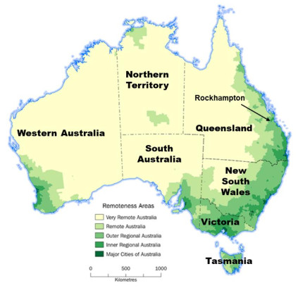
Two hand-on workshops on social media apps were conducted for the Year-12 students from two schools, one from a regional city and the other from a remote community, in a computer laboratory on the Rockhampton campus at Central Queensland University before the COVID-19 pandemic. The school in the regional city offered a specialist Digital Technologies Curriculum (DTC) to students in Years 11 & 12 whereas the remote school did not offer a similar DTC to students in Years 11 & 12. Statistical analyses of the students' responses to two casual questions during the workshop indicated that firstly the hands-on activities improved all students' general IT knowledge, and secondly the Year-12 students from the regional city were more determined to undertake tertiary IT education than the students from the remote school. Therefore, it is recommended that a mandatory specialist DTC for students in Years 11 & 12 in ALL schools should be included in the national curriculum in the future. Implications of these findings on improving the participation rate of post-secondary education in Australian regional communities are also discussed in this article. In particular, regional universities can play a unique role in producing "IT allrounders" to meet the needs of the regional communities through collaborations with governments, secondary schools, regional industries and businesses.
Citation: Wei Li, William Guo. Analysing responses of Year-12 students to a hands-on IT workshop: Implications for increasing participation in tertiary IT education in regional Australia[J]. STEM Education, 2023, 3(1): 43-56. doi: 10.3934/steme.2023004
Two hand-on workshops on social media apps were conducted for the Year-12 students from two schools, one from a regional city and the other from a remote community, in a computer laboratory on the Rockhampton campus at Central Queensland University before the COVID-19 pandemic. The school in the regional city offered a specialist Digital Technologies Curriculum (DTC) to students in Years 11 & 12 whereas the remote school did not offer a similar DTC to students in Years 11 & 12. Statistical analyses of the students' responses to two casual questions during the workshop indicated that firstly the hands-on activities improved all students' general IT knowledge, and secondly the Year-12 students from the regional city were more determined to undertake tertiary IT education than the students from the remote school. Therefore, it is recommended that a mandatory specialist DTC for students in Years 11 & 12 in ALL schools should be included in the national curriculum in the future. Implications of these findings on improving the participation rate of post-secondary education in Australian regional communities are also discussed in this article. In particular, regional universities can play a unique role in producing "IT allrounders" to meet the needs of the regional communities through collaborations with governments, secondary schools, regional industries and businesses.

| [1] | Regional Education Expert Advisory Group (REEAG), National Regional, Rural and Remote Tertiary Education Strategy—Final Report. 2019, Canberra, Australia: Commonwealth of Australia. |
| [2] |
Guo, W., Exploratory case study on solving word problems involving triangles by pre-service mathematics teachers in a regional university in Australia. Mathematics, 2022, 10: 3786. https://doi.org/10.3390/math10203786 doi: 10.3390/math10203786

|
| [3] | Wilson, S., Lyons, T. and Quinn, F., Should I stay or should I go? Rural and remote students in first year university stem courses. Australian and International Journal of Rural Education, 2013, 23(2): 77–88. |
| [4] |
Fraser, S., Beswick, K. and Crowley, S., Responding to the demands of the STEM education agenda: The experiences of primary and secondary teachers from rural, regional and remote Australia. Journal of Research in STEM Education, 2019, 5(1): 40–59. doi: 10.51355/jstem.2019.62
|
| [5] |
Murphy, S., Science education success in a rural Australian school: Practices and arrangements contributing to high senior science enrolments and achievement in an isolated rural school. Research in Science Education, 2020, 52: 325–337. https://doi.org/10.1007/s11165-020-09947-5 doi: 10.1007/s11165-020-09947-5
|
| [6] |
Allen, K.A., Cordoba, B.G., Parks, A., Arslan, G., Does socioeconomic status moderate the relationship between school belonging and school-related factors in Australia? Child Indicators Research, 2022, 15: 1741–1759. https://doi.org/10.1007/s12187-022-09927-3 doi: 10.1007/s12187-022-09927-3
|
| [7] | Courtney, L., Anderson, N., Do rural and regional students in Queensland experience an ICT 'turn-off' in the early high school years? Australian Educational Computing, 2010, 25(2): 7–11. |
| [8] |
Vichie, K., Higher education and digital media in regional Australia: The current situation for youth. Australian and International Journal of Rural Education, 2017, 27(1): 29–42. doi: 10.47381/aijre.v27i1.107
|
| [9] | Flack, C.B., Walker, L., Bickerstaff, A., Margetts, C., Socioeconomic disparities in Australian schooling during the COVID-19 pandemic. 2020, Melbourne, Australia: Pivot Professional Learning. |
| [10] |
Guo, W., Li, W., A workshop on social media apps for Year-10 students: An exploratory case study on digital technology education in regional Australia. Online Journal of Communication and Media Technologies, 2022, 12: e202222. https://doi.org/10.30935/ojcmt/12237 doi: 10.30935/ojcmt/12237
|
| [11] | ACARA., The Australian curriculum: Digital technologies (v 8.4) for Years 9 & 10. Australian Curriculum, Assessment and Reporting Authority. Available from: https://www.australiancurriculum.edu.au/f-10-curriculum/technologies/digital-technologies/ |
| [12] | Boone, H.N., Boone, D.A., Analyzing Likert data. Journal of Extension, 2012, 50(2): Article 2TOT2. |
| [13] | Joshi, A., Kale, S., Chandel, S., Pal, D.K., Likert scale: Explored and explained. British Journal of Applied Science & Technology, 2015, 7(4): 396–403. |
| [14] | Duncan-Howell, J., Digital mismatch: Expectations and realities of digital competency amongst pre-service education students. Australasian Journal of Educational Technology, 2012, 28(5): 827–840. |
| [15] |
Considine, G., Zappalà, G., The influence of social and economic disadvantage in the academic performance of school students in Australia. Journal of Sociology, 2002, 38(2): 129–148. https://doi.org/10.1177/144078302128756543. doi: 10.1177/144078302128756543
|
| [16] | Queensland Audit Office, Enabling Digital Learning (Report 1: 2021-22). 2021, Brisbane, Australia: The State of Queensland |
| [17] |
Gibson, S., Patfield, S., Gore, J.M., Fray, L., Aspiring to higher education in regional and remote Australia: the diverse emotional and material realities shaping young people's futures. Australian Educational Researcher, 2022, 49: 1105–1124. https://doi.org/10.1007/s13384-021-00463-7 doi: 10.1007/s13384-021-00463-7
|
| [18] |
Guo, W., Li, W., Dodd, R., Gide, E., The trifecta for curriculum sustainability in Australian universities. STEM Education, 2021, 1(1): 1–16. https://doi.org/10.3934/steme.2021001 doi: 10.3934/steme.2021001
|


Figures(4) / Tables(5)
Wei Li, William Guo. Analysing responses of Year-12 students to a hands-on IT workshop: Implications for increasing participation in tertiary IT education in regional Australia[J]. STEM Education, 2023, 3(1): 43-56. doi: 10.3934/steme.2023004


 DownLoad: