While there are works on best practices in teaching, there is a lack of literature that concerns the associated leadership aspect. However, contemporary online educators largely play the role of leaders consciously or unconsciously. Further, STEM and technical social science subjects like finance can be related to a substantial cognitive load if instructions are poorly designed, and more so in an online context where students and educators may not have a close connection. This perspective article, drawing on the author's own experience as a successful online educator with consistently high student satisfaction scores and multiple teaching awards and referring to literature, conceptualizes good online teaching practices in technical disciplines across two dimensions – virtual leadership and cognitive load management. The perspective then suggests strategies particularly applicable in technical disciplines to achieve satisfactory learning outcomes. It is acknowledged that online delivery and style of teaching adopted by educators can be subjective and dependent on context. However, the practices suggested, including communicating expectations, developing trust-relationship with students, adaptations beyond conventional teaching and textbook, and designing and sequencing resources while considering cognitive load management, may positively impact online students' learning experience in STEM and technical social science disciplines.
Citation: Tasadduq Imam. Good practices of delivery and teaching leadership for online educators in technical disciplines: A perspective[J]. STEM Education, 2021, 1(2): 92-103. doi: 10.3934/steme.2021007
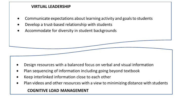
While there are works on best practices in teaching, there is a lack of literature that concerns the associated leadership aspect. However, contemporary online educators largely play the role of leaders consciously or unconsciously. Further, STEM and technical social science subjects like finance can be related to a substantial cognitive load if instructions are poorly designed, and more so in an online context where students and educators may not have a close connection. This perspective article, drawing on the author's own experience as a successful online educator with consistently high student satisfaction scores and multiple teaching awards and referring to literature, conceptualizes good online teaching practices in technical disciplines across two dimensions – virtual leadership and cognitive load management. The perspective then suggests strategies particularly applicable in technical disciplines to achieve satisfactory learning outcomes. It is acknowledged that online delivery and style of teaching adopted by educators can be subjective and dependent on context. However, the practices suggested, including communicating expectations, developing trust-relationship with students, adaptations beyond conventional teaching and textbook, and designing and sequencing resources while considering cognitive load management, may positively impact online students' learning experience in STEM and technical social science disciplines.

| [1] |
The making of an exemplary online educator. Distance Education (2011) 32: p.101-118. 
|
| [2] |
Twelve tips for using social media as a medical educator. Medical Teacher (2014) 36: p.284-290.
|
| [3] |
Training Online Technical Communication Educators to Teach with Social Media: Best Practices and Professional Recommendations. Technical Communication Quarterly (2017) 26: p.344-359.
|
| [4] |
Online educators' recommendations for teaching online: Crowdsourcing in action. Open Praxis (2018) 10: p.79-89.
|
| [5] |
Improving Online Teaching by Using Established Best Classroom Teaching Practices. The Journal of Continuing Education in Nursing (2016) 47: p.222-227.
|
| [6] | Bain, K., What the Best College Teachers Do, 2004. Harvard University Press. |
| [7] |
Use and Acceptance of Social Media Among Health Educators. American Journal of Health Education (2011) 42: p.197-204.
|
| [8] |
Novice online educator conceptual frameworks: a mental model exploration of mindful learning design. Educational Media International (2019) 56: p.14-43.
|
| [9] | Leibold, N., and Schwarz, L. M., The Art of Giving Online Feedback. Journal of Effective Teaching, 2015. 15(1): p. 34–46. ISSN: 1935-7869. |
| [10] | Chickering, A. W., and Gamson, Z. F., Seven Principles for Good Practice in Undergraduate Education. AAHE Bulletin, 1987. p. 3–7. |
| [11] | Imam, T., Teaching online is leading online: some success strategies. Campus Review, 2020 (July 08). Available: https://www.campusreview.com.au/2020/07/teaching-online-is-leading-online-some-success-strategies/. |
| [12] | Sweller, J., CHAPTER TWO - Cognitive Load Theory, in Psychology of Learning and Motivation, eds. Mestre, J. P., and Ross, B. H., 2011. Academic Press, p. 37–76. |
| [13] |
Cognitive load theory, learning difficulty, and instructional design. Learning and Instruction (1994) 4: p.295-312.
|
| [14] |
Cognitive load during problem solving: Effects on learning. Cognitive Science (1988) 12: p.257-285.
|
| [15] | Textbook Readability and Student Performance in Online Introductory Corporate Finance Classes. Journal of Educators Online (2015) 12: p.35-49. |
| [16] |
Humour Applied to STEM Education. Systems Research and Behavioral Science (2017) 34: p.216-226.
|
| [17] |
Value of Case-Based Learning within STEM Courses: Is It the Method or Is It the Student?. CBE—Life Sciences Education (2020) 19: p.a.
|
| [18] | Maj, S. P., and Nuangjamnong, C., Using Cognitive Load Optimiztion to teach STEM Disciplines to Business Students, in 2020 IEEE International Conference on Teaching, Assessment, and Learning for Engineering (TALE), 2020. Takamatsu, Japan, p. 428–435. |
| [19] |
Leading Virtual Teams. Academy of Management Perspectives (2007) 21: p.60-70.
|
| [20] | Schmidt, G., Virtual Leadership: An Important Leadership Context. Industrial and Organizational Psychology, 2014. 7 doi: 10.1111/iops.12129. |
| [21] |
Leadership in virtual teams: A multilevel perspective. Human Resource Management Review (2017) 27: p.648-659.
|
| [22] |
Paradoxical Virtual Leadership: Reconsidering Virtuality Through a Paradox Lens. Group & Organization Management (2018) 43: p.752-786.
|
| [23] | Mangente, B. P., Does Virtual Leadership Style Matter? An Examination of Leadership Styles of Effective Virtual Teams in the U.S. Navy, Ph.D., Alliant International University, (2020). |
| [24] |
246 reasons to cheat: An analysis of students' reasons for seeking to outsource academic work. Computers & Education (2019) 134: p.98-107.
|
| [25] |
Contract cheating: a survey of Australian university students. Studies in Higher Education (2019) 44: p.1837-1856.
|
| [26] | Bligh, M. C., Leadership and Trust, in Leadership Today: Practices for Personal and Professional Performance, eds. Marques, J., and Dhiman, S., 2017. Cham: Springer International Publishing, p. 21–42. |
| [27] |
The development of trust in virtual leader-follower relationships. Qualitative Research in Organizations and Management: An International Journal (2019) 15: p.279-295.
|
| [28] |
Undergraduate student responses to feedback: expectations and experiences. Studies in Higher Education (2016) 41: p.2078-2094.
|
| [29] |
Assessment, feedback and marking guides in distance education. Open Learning: The Journal of Open, Distance and e-Learning (2011) 26: p.67-78.
|
| [30] | Global Leadership and Diversity. Journal of Educational and Social Research (2015) 5: p.161-168. |
| [31] |
Learning Styles and Learning Spaces: Enhancing Experiential Learning in Higher Education. Academy of Management Learning & Education (2005) 4: p.193-212.
|
| [32] |
Critically reflective practice. Journal of Continuing Education in the Health Professions (1998) 18: p.197-205.
|
| [33] | Barnes, K., Marateo, R. C., and Ferris, S. P., Teaching and Learning with the Net Generation. Innovate: Journal of Online Education, 2007. 3(4): Online. ISSN: 1552-3233. |
| [34] |
Generation Y students : appropriate learning styles and teaching approaches in the economic and management sciences faculty. South African Journal of Higher Education (2009) 23: p.1039-1058.
|
| [35] |
Cognitive Architecture and Instructional Design. Educational Psychology Review (1998) 10: p.251-296.
|
| [36] |
Cognitive Load Theory: How Many Types of Load Does It Really Need?. Educational Psychology Review (2011) 23: p.1-19.
|
| [37] |
Nine Ways to Reduce Cognitive Load in Multimedia Learning. Educational Psychologist (2003) 38: p.43-52.
|
| [38] |
How do instructional designers manage learners' cognitive load? An examination of awareness and application of strategies. Educational Technology Research and Development (2019) 67: p.199-245.
|
| [39] |
The impact of complexity on the expertise reversal effect: experimental evidence from testing accounting students. Educational Psychology (2016) 36: p.1868-1885.
|
| [40] |
Transactional Presence as a Critical Predictor of Success in Distance Learning. Distance Education (2003) 24: p.69-86.
|
| [41] | Guo, P. J., Kim, J., and Rubin, R., How video production affects student engagement: an empirical study of MOOC videos, in Proceedings of the First ACM Conference on Learning @ Scale Conference, 2014. New York, NY, USA: Association for Computing Machinery, p. 41–50. |
| [42] |
The changing role of the educational video in higher distance education. The International Review of Research in Open and Distributed Learning (2017) 18:.
|
| [43] |
The Importance of Instructor Clarity and Its Effect on Student Learning: Facilitating Elaboration by Reducing Cognitive Load. Communication Reports (2016) 29: p.152-162.
|
Figures(1)
Tasadduq Imam. Good practices of delivery and teaching leadership for online educators in technical disciplines: A perspective[J]. STEM Education, 2021, 1(2): 92-103. doi: 10.3934/steme.2021007


 DownLoad: