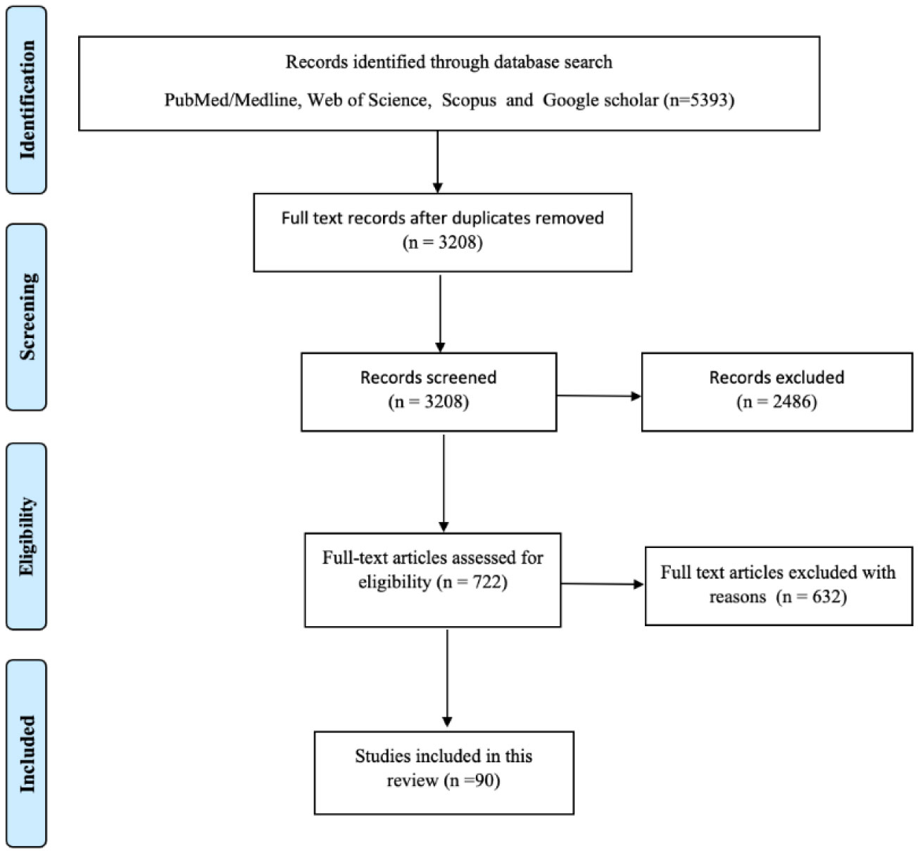
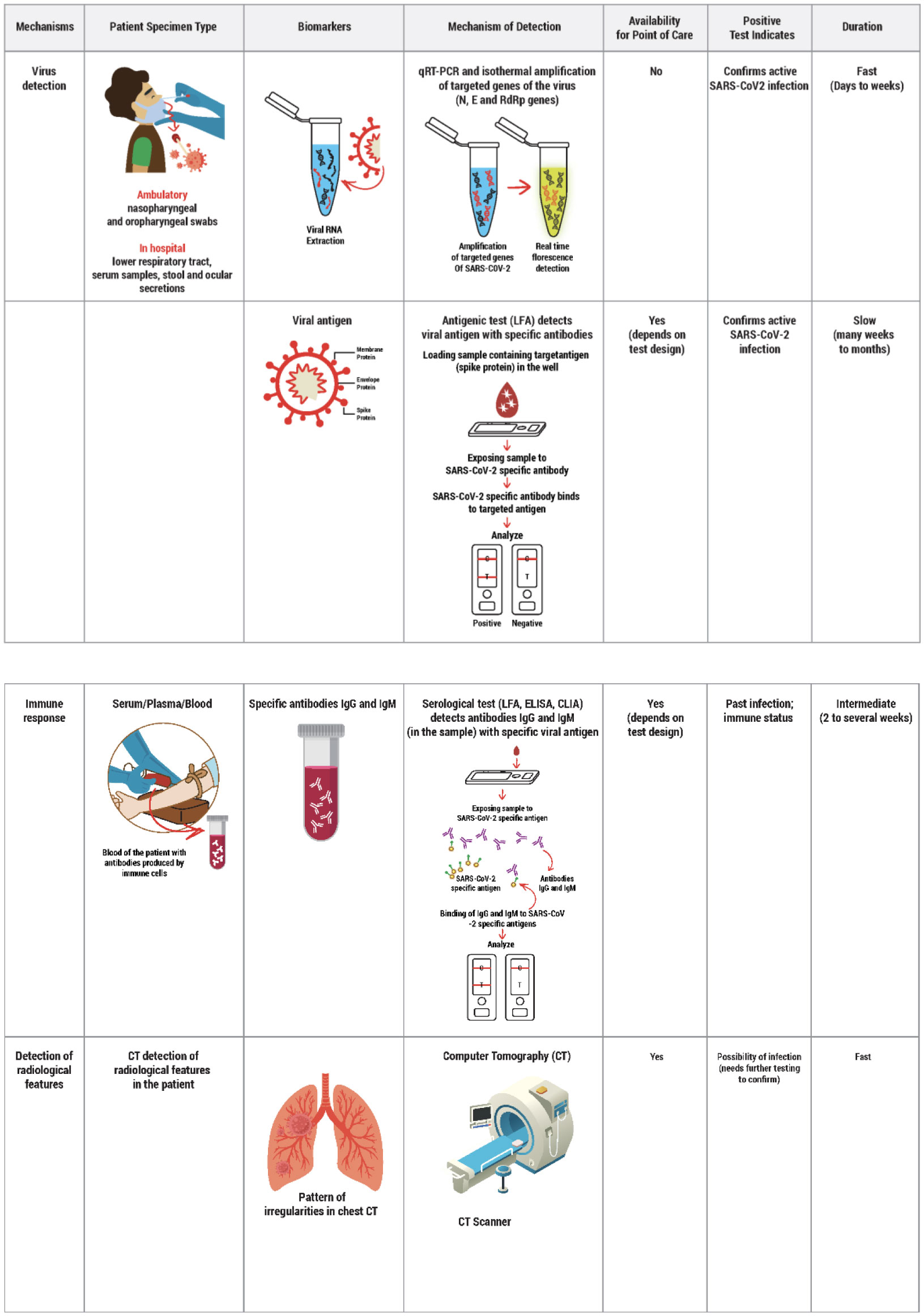
COVID-19 is caused by SARS-CoV-2, which originated in Wuhan, Hubei province, Central China, in December 2019 and since then has spread rapidly, resulting in a severe pandemic. The infected patient presents with varying non-specific symptoms requiring an accurate and rapid diagnostic tool to detect SARS-CoV-2. This is followed by effective patient isolation and early treatment initiation ranging from supportive therapy to specific drugs such as corticosteroids, antiviral agents, antibiotics, and the recently introduced convalescent plasma. The development of an efficient vaccine has been an on-going challenge by various nations and research companies. A literature search was conducted in early December 2020 in all the major databases such as Medline/PubMed, Web of Science, Scopus and Google Scholar search engines. The findings are discussed in three main thematic areas namely diagnostic approaches, therapeutic options, and potential vaccines in various phases of development. Therefore, an effective and economical vaccine remains the only retort to combat COVID-19 successfully to save millions of lives during this pandemic. However, there is a great scope for further research in discovering cost-effective and safer therapeutics, vaccines and strategies to ensure equitable access to COVID-19 prevention and treatment services.
Citation: Srikanth Umakanthan, Vijay Kumar Chattu, Anu V Ranade, Debasmita Das, Abhishekh Basavarajegowda, Maryann Bukelo. A rapid review of recent advances in diagnosis, treatment and vaccination for COVID-19[J]. AIMS Public Health, 2021, 8(1): 137-153. doi: 10.3934/publichealth.2021011
COVID-19 is caused by SARS-CoV-2, which originated in Wuhan, Hubei province, Central China, in December 2019 and since then has spread rapidly, resulting in a severe pandemic. The infected patient presents with varying non-specific symptoms requiring an accurate and rapid diagnostic tool to detect SARS-CoV-2. This is followed by effective patient isolation and early treatment initiation ranging from supportive therapy to specific drugs such as corticosteroids, antiviral agents, antibiotics, and the recently introduced convalescent plasma. The development of an efficient vaccine has been an on-going challenge by various nations and research companies. A literature search was conducted in early December 2020 in all the major databases such as Medline/PubMed, Web of Science, Scopus and Google Scholar search engines. The findings are discussed in three main thematic areas namely diagnostic approaches, therapeutic options, and potential vaccines in various phases of development. Therefore, an effective and economical vaccine remains the only retort to combat COVID-19 successfully to save millions of lives during this pandemic. However, there is a great scope for further research in discovering cost-effective and safer therapeutics, vaccines and strategies to ensure equitable access to COVID-19 prevention and treatment services.

| [1] |
Pooladanda V, Thatikonda S, Godugu C (2020) The current understanding and potential therapeutic options to combat COVID-19. Life Sci 254: 117765. doi: 10.1016/j.lfs.2020.117765

|
| [2] |
Wang H, Li X, Li T, et al. (2020) The genetic sequence, origin, and diagnosis of SARS-CoV-2. Eur J Clin Microbiol Infect Dis 39: 1629-1635. doi: 10.1007/s10096-020-03899-4
|
| [3] |
Li H, Liu SM, Yu XH, et al. (2020) Coronavirus disease 2019 (COVID-19): current status and future perspectives. Int J Antimicrob Agents 55: 105951. doi: 10.1016/j.ijantimicag.2020.105951
|
| [4] | Wu J, Deng W, Li S, et al. (2020) Advances in research on ACE2 as a receptor for 2019-nCoV. Cell Mol Life Sci 1-14. |
| [5] | Umakanthan S, Sahu P, Ranade AV, et al. (2020) Origin, transmission, diagnosis and management of coronavirus disease 2019 (COVID-19). Postgrad Med J 96: 753-758. |
| [6] |
Fu L, Wang B, Yuan T, et al. (2020) Clinical characteristics of coronavirus disease 2019 (COVID-19) in China: A systematic review and meta-analysis. J Infect 80: 656-665. doi: 10.1016/j.jinf.2020.03.041
|
| [7] |
Iyer M, Jayaramayya K, Subramaniam MD, et al. (2020) COVID-19: an update on diagnostic and therapeutic approaches. BMB Rep 53: 191-205. doi: 10.5483/BMBRep.2020.53.4.080
|
| [8] |
Touma M (2020) COVID-19: molecular diagnostics overview. J Mol Med (Berl) 98: 947-954. doi: 10.1007/s00109-020-01931-w
|
| [9] |
Huang C, Wang Y, Li X, et al. (2020) Clinical features of patients infected with 2019 novel coronavirus in Wuhan, China. Lancet 395: 497-506. doi: 10.1016/S0140-6736(20)30183-5
|
| [10] |
Zhou F, Yu T, Du R, et al. (2020) Clinical course and risk factors for mortality of adult inpatients with COVID-19 in Wuhan, China: a retrospective cohort study. Lancet 395: 1054-1062. doi: 10.1016/S0140-6736(20)30566-3
|
| [11] | Zheng F, Tang W, Li H, et al. (2020) Clinical characteristics of 161 cases of corona virus disease 2019 (COVID-19) in Changsha. Eur Rev Med Pharmacol Sci 24: 3404-3410. |
| [12] |
Chu DKW, Pan Y, Cheng SMS, et al. (2020) Molecular diagnosis of a novel coronavirus (2019-nCoV) causing an outbreak of pneumonia. Clin Chem 66: 549-555. doi: 10.1093/clinchem/hvaa029
|
| [13] |
Loeffelholz MJ, Tang YW (2020) Laboratory diagnosis of emerging human coronavirus infections—the state of the art. Emerg Microbes Infect 9: 747-756. doi: 10.1080/22221751.2020.1745095
|
| [14] |
Emery SL, Erdman DD, Bowen MD, et al. (2004) Real-time reverse transcription-polymerase chain reaction assay for SARS-associated Coronavirus. Emerg Infect Dis 10: 311-316. doi: 10.3201/eid1002.030759
|
| [15] |
Wölfel R, Corman VM, Guggemos W, et al. (2020) Virological assessment of hospitalized patients with COVID-2019. Nature 581: 465-469. doi: 10.1038/s41586-020-2196-x
|
| [16] |
Hans R, Marwaha N (2014) Nucleic acid testing-benefits and constraints. Asian J Transfus Sci 8: 2-3. doi: 10.4103/0973-6247.126679
|
| [17] | La Marca A, Capuzzo M, Paglia T, et al. (2020) Testing for SARS-CoV-2 (COVID-19): a systematic review and clinical guide to molecular and serological in-vitro diagnostic assays. Reprod Biomed Online . |
| [18] | Doi A, Iwata K, Kuroda H, et al. (2020) Estimation of seroprevalence of novel coronavirus disease (COVID-19) using preserved serum at an outpatient setting in Kobe, Japan: A cross-sectional study. medRxiv . |
| [19] | Li Z, Yi Y, Luo X, et al. (2020) Development and Clinical Application of A Rapid IgM-IgG Combined Antibody Test for SARS-CoV-2 Infection Diagnosis. J Med Virol 27: 25727. |
| [20] | Liu R, Liu X, Han H, et al. The comparative superiority of IgM-IgG antibody test to real-time reverse transcriptase PCR detection for SARS-CoV-2 infection diagnosis 2020 (2020) .Available from: https://doi.org/10.1101/2020.03.28.20045765. |
| [21] |
Grant BD, Anderson CE, Williford JR, et al. (2020) SARS-CoV-2 Coronavirus Nucleocapsid Antigen-Detecting Half-Strip Lateral Flow Assay Toward the Development of Point of Care Tests Using Commercially Available Reagents. Anal Chem 92: 11305-11309. doi: 10.1021/acs.analchem.0c01975
|
| [22] |
Burki TK (2020) Testing for COVID-19. Lancet Respir Med 8: e63-e64. doi: 10.1016/S2213-2600(20)30247-2
|
| [23] | Chen H, Ai L, Lu H, et al. (2020) Clinical and imaging features of COVID-19. Radiol Infect Dis . |
| [24] |
Singh AK, Majumdar S, Singh R, et al. (2020) Role of corticosteroid in the management of COVID-19: A systemic review and a Clinician's perspective. Diabetes Metab Syndr 14: 971-978. doi: 10.1016/j.dsx.2020.06.054
|
| [25] |
Perez A, Jansen-Chaparro S, Saigi I, et al. (2014) Glucocorticoid-induced hyperglycemia. J Diabetes 6: 9-20. doi: 10.1111/1753-0407.12090
|
| [26] |
Singh AK, Singh A, Singh R, et al. (2020) Remdesivir in COVID-19: A critical review of pharmacology, pre-clinical and clinical studies. Diabetes Metab Syndr 14: 641-648. doi: 10.1016/j.dsx.2020.05.018
|
| [27] |
Bhatraju PK, Ghassemieh BJ, Nichols M, et al. (2020) Covid-19 in Critically Ill Patients in the Seattle Region—Case Series. N Engl J Med 382: 2012-2022. doi: 10.1056/NEJMoa2004500
|
| [28] |
Singh AK, Singh A, Shaikh A, et al. (2020) Chloroquine and hydroxychloroquine in the treatment of COVID-19 with or without diabetes: A systematic search and a narrative review with a special reference to India and other developing countries. Diabetes Metab Syndr 14: 241-246. doi: 10.1016/j.dsx.2020.03.011
|
| [29] |
Moore N (2020) Chloroquine for COVID-19 Infection. Drug Saf 43: 393-394. doi: 10.1007/s40264-020-00933-4
|
| [30] | Owa AB, Owa OT (2020) Lopinavir/ritonavir use in Covid-19 infection: is it completely non-beneficial? J Microbiol Immunol Infect . |
| [31] |
Uzunova K, Filipova E, Pavlova V, et al. (2020) Insights into antiviral mechanisms of remdesivir, lopinavir/ritonavir and chloroquine/hydroxychloroquine affecting the new SARS-CoV-2. Biomed Pharmacother 131: 110668. doi: 10.1016/j.biopha.2020.110668
|
| [32] | Heidary F, Gharebaghi R, et al. (2020) Ivermectin: a systematic review from antiviral effects to COVID-19 complementary regimen. J Antibiot (Tokyo) 1-10. |
| [33] | Gupta D, Sahoo AK, Singh A (2020) Ivermectin: potential candidate for the treatment of Covid 19. Braz J Infect Dis . |
| [34] |
Coomes EA, Haghbayan H (2020) Favipiravir, an antiviral for COVID-19? J Antimicrob Chemother 75: 2013-2014. doi: 10.1093/jac/dkaa171
|
| [35] | Cai Q, Yang M, Liu D, et al. (2020) Experimental Treatment with Favipiravir for COVID-19: An Open-Label Control Study. Engineering (Beijing) . |
| [36] | Wu R, Wang L, Kuo HD, et al. (2020) An Update on Current Therapeutic Drugs Treating COVID-19. Curr Pharmacol Rep 1-15. |
| [37] |
Huttner BD, Catho G, Pano-Pardo JR, et al. (2020) COVID-19: don't neglect anti-microbial stewardship principles!. Clin Microbiol Infect 26: 808-810. doi: 10.1016/j.cmi.2020.04.024
|
| [38] |
Rawson TM, Ming D, Ahmad R, et al. (2020) Anti-microbial use, drug-resistant infections and COVID-19. Nat Rev Microbiol 18: 409-410. doi: 10.1038/s41579-020-0395-y
|
| [39] | Cai X, Ren M, Chen F, et al. (2020) Blood transfusion during the COVID-19 outbreak. Blood Transfus 18: 79-82. |
| [40] | Kumar S, Sharma V, Priya K (2020) Battle against COVID-19: Efficacy of Convalescent Plasma as an emergency therapy. Am J Emerg Med . |
| [41] |
Mair-Jenkins J, Saavedra-Campos M, Baillie JK (2015) The effectiveness of convalescent plasma and hyperimmune immunoglobulin for the treatment of severe acute respiratory infections of viral etiology: a systematic review and exploratory meta-analysis. J Infect Dis 211: 80-90. doi: 10.1093/infdis/jiu396
|
| [42] | Valk SJ, Piechotta V, Chai KL, et al. (2020) Convalescent plasma or hyperimmune immunoglobulin for people with COVID-19: a rapid review. Cochrane Db Syst Rev 5: CD013600. |
| [43] | Hartman WR, Hess AS, Connor JP Hospitalized COVID-19 Patients treated with Convalescent Plasma in a Mid-size City in the Midwest (2020) .Available from: https://www.researchgate.net/publication/346772157_Hospitalized_COVID-19_Patients_treated_with_Convalescent_Plasma_in_a_Mid-size_City_in_the_Midwest. |
| [44] |
Li L, Zhang W, Hu Y, et al. (2020) Effect of Convalescent Plasma Therapy on Time to Clinical Improvement in Patients With Severe and Life-threatening COVID-19: A Randomized Clinical Trial. JAMA 324: 460-470. doi: 10.1001/jama.2020.10044
|
| [45] |
Rajarshi K, Chatterjee A, Ray S (2020) Combating COVID-19 with Mesenchymal Stem Cell therapy. Biotechnol Rep (Amst) 26: e00467. doi: 10.1016/j.btre.2020.e00467
|
| [46] |
Golchin A, Seyedjafari E, Ardeshirylajimi A (2020) Mesenchymal Stem Cell Therapy for COVID-19: Present or Future. Stem Cell Rev Rep 16: 427-433. doi: 10.1007/s12015-020-09973-w
|
| [47] |
Golchin A, Farahany TZ, Khojasteh A, et al. (2018) The clinical trials of Mesenchymal stem cell therapy in skin diseases: An update and concise review. Curr Stem Cell Res Ther 14: 22-33. doi: 10.2174/1574888X13666180913123424
|
| [48] | Kewan T, Covut F, Al-Jaghbeer MJ, et al. (2020) Tocilizumab for treatment of patients with severe COVID–19: A retrospective cohort study. E Clin Med 100418. |
| [49] | Guaraldi G, Meschiari M, Cozzi-Lepri A, et al. (2020) Tocilizumab in patients with severe COVID-19: a retrospective cohort study. Lancet Rheumatol 2. |
| [50] | Cantini F, Niccoli L, Nannini C, et al. (2020) Beneficial impact of Baricitinib in COVID-19 moderate pneumonia; multicentre study. J Infect . |
| [51] |
Cantini F, Niccoli L, Matarrese D, et al. (2020) Baricitinib therapy in COVID-19: A pilot study on safety and clinical impact. J Infect 81: 318-356. doi: 10.1016/j.jinf.2020.04.017
|
| [52] |
Maoujoud O, Asserraji M, Ahid S, et al. (2020) Anakinra for patients with COVID-19. Lancet Rheumatol 2: e383. doi: 10.1016/S2665-9913(20)30177-6
|
| [53] |
Filocamo G, Mangioni D, Tagliabue P, et al. (2020) Use of anakinra in severe COVID-19: A case report. Int J Infect Dis 96: 607-609. doi: 10.1016/j.ijid.2020.05.026
|
| [54] | Kow CS, Hasan SS (2020) Use of low-molecular-weight heparin in COVID-19 patients. J Vasc Surg Venous Lymphat Disord . |
| [55] | Costanzo L, Palumbo FP, Ardita G, et al. (2020) Coagulopathy, thromboembolic complications, and the use of heparin in COVID-19 pneumonia. J Vasc Surg Venous Lymphat Disord . |
| [56] | Turshudzhyan A (2020) Anticoagulation Options for Coronavirus Disease 2019 (COVID-19)-Induced Coagulopathy. Cureus 12: e8150. |
| [57] |
Boretti A, Banik BK (2020) Intravenous Vitamin C for reduction of cytokines storm in Acute Respiratory Distress Syndrome. PharmaNutrition 12: 100190. doi: 10.1016/j.phanu.2020.100190
|
| [58] |
Simonson W (2020) Vitamin C and Coronavirus. Geriatr Nurs 41: 331-332. doi: 10.1016/j.gerinurse.2020.05.002
|
| [59] |
Hemilä H (2003) Vitamin C and SARS coronavirus. J Antimicrob Chemother 52: 1049-1050. doi: 10.1093/jac/dkh002
|
| [60] | World Health Organization Draft landscape of COVID-19 candidate vaccines (2020) .Available from: https://www.who.int/who-documents-detail/draft-landscape-of-covid-19-candidate-vaccines. |
| [61] |
Day M (2020) Covid-19: four fifths of cases are asymptomatic, China figures indicate. BMJ 369: 1375. doi: 10.1136/bmj.m1375
|
| [62] |
Sutton D, Fuchs K, D'Alton M, et al. (2020) Universal Screening for SARS-CoV-2 in Women Admitted for Delivery. N Engl J Med 382: 2163-2164. doi: 10.1056/NEJMc2009316
|
| [63] |
Mizumoto K, Kagaya K, Zarebski A, et al. (2020) Estimating the asymptomatic proportion of coronavirus disease 2019 (COVID-19) cases on board the Diamond Princess cruise ship, Yokohama, Japan, 2020. Euro Surveill 25: 2000180. doi: 10.2807/1560-7917.ES.2020.25.10.2000180
|
| [64] |
Wrapp D, Wang N, Corbett KS, et al. (2020) Cryo-EM structure of the 2019-nCoV spike in the prefusion conformation. Science 367: 1260-1263. doi: 10.1126/science.abb2507
|
| [65] |
Andersen KG, Rambaut A, Lipkin WI, et al. (2020) The proximal origin of SARS-CoV-2. Nat Med 26: 450-452. doi: 10.1038/s41591-020-0820-9
|
| [66] |
Benvenuto D, Giovanetti M, Ciccozzi A, et al. (2020) The 2019-new coronavirus epidemic: Evidence for virus evolution. J Med Virol 92: 455-459. doi: 10.1002/jmv.25688
|
| [67] |
Yan R, Zhang Y, Li Y, et al. (2020) Structural basis for the recognition of SARS-CoV-2 by full-length human ACE2. Science 367: 1444-1448. doi: 10.1126/science.abb2762
|
| [68] |
Enjuanes L, Zuñiga S, Castaño-Rodriguez C, et al. (2016) Molecular Basis of Coronavirus Virulence and Vaccine Development. Adv Virus Res 96: 245-286. doi: 10.1016/bs.aivir.2016.08.003
|
| [69] |
Song Z, Xu Y, Bao L, et al. (2019) From SARS to MERS, Thrusting Coronaviruses into the Spotlight. Viruses 11: 59. doi: 10.3390/v11010059
|
| [70] | Wu F, Wang A, Liu M, et al. (2020) Neutralizing antibody responses to SARS-CoV-2 in a COVID-19 recovered patient cohort and their implications. medRxiv . |
| [71] |
Thi Nhu Thao T, Labroussaa F, Ebert N, et al. (2020) Rapid reconstruction of SARS-CoV-2 using a synthetic genomics platform. Nature 582: 561-565. doi: 10.1038/s41586-020-2294-9
|
| [72] |
Xie X, Muruato A, Lokugamage KG, et al. (2020) An Infectious cDNA Clone of SARS-CoV-2. Cell Host Microbe 27: 841-848. doi: 10.1016/j.chom.2020.04.004
|
| [73] |
Dicks MD, Spencer AJ, Edwards NJ, et al. (2012) A novel chimpanzee adenovirus vector with low human seroprevalence: improved systems for vector derivation and comparative immunogenicity. PLoS One 7: e40385. doi: 10.1371/journal.pone.0040385
|
| [74] |
Fausther-Bovendo H, Kobinger GP (2014) Pre-existing immunity against Advectors. Hum Vaccines Immunother 10: 2875-2884. doi: 10.4161/hv.29594
|
| [75] |
Alberer M, Gnad-Vogt U, Hong HS, et al. (2017) Safety and immunogenicity of a mRNA rabies vaccine in healthy adults: an open-label, non-randomized, prospective, first-in-human phase 1 clinical trial. Lancet 390: 1511-1520. doi: 10.1016/S0140-6736(17)31665-3
|
| [76] |
Smith TRF, Patel A, Ramos S, et al. (2020) Immunogenicity of a DNA vaccine candidate for COVID-19. Nat Commun 11: 2601. doi: 10.1038/s41467-020-16505-0
|
| [77] | BIONTECH BioNTech and Pfizer announce regulatory approval from German authority Paul-Ehrlich-Institut to commence first clinical trial of COVID-19 vaccine candidates (2020) .Available from: https://investors.biontech.de/node/7431/pdf. |
| [78] |
Takashima Y, Osaki M, Ishimaru Y, et al. (2011) Artificial molecular clamp: A novel device for synthetic polymerases. Angew Chem Int Ed 50: 7524-7528. doi: 10.1002/anie.201102834
|
| [79] |
Singh K, Mehta S (2016) The clinical development process for a novel preventive vaccine: An overview. J Postgrad Med 62: 4-11. doi: 10.4103/0022-3859.173187
|
| [80] |
Wang Q, Zhang L, Kuwahara K, et al. (2016) Immunodominant SARS Coronavirus Epitopes in Humans Elicited both Enhancing and Neutralizing Effects on Infection in Non-human Primates. ACS Infect Dis 2: 361-376. doi: 10.1021/acsinfecdis.6b00006
|
| [81] | de Sousa E, Ligeiro D, Lérias JR, et al. (2020) Mortality in COVID-19 disease patients: Correlating Association of Major histocompatibility complex (MHC) with severe acute respiratory syndrome 2 (SARS-CoV-2) variants. Int J Infect Dis . |
| [82] |
Li H, Liu SM, Yu XH, et al. (2020) Coronavirus disease 2019 (COVID-19): current status and future perspectives. Int J Antimicrob Agents 55: 105951. doi: 10.1016/j.ijantimicag.2020.105951
|
| [83] |
Deb B, Shah H, Goel S (2020) Current global vaccine and drug efforts against COVID-19: Pros and cons of bypassing animal trials. J Biosci 45: 82. doi: 10.1007/s12038-020-00053-2
|
| [84] |
Abd El-Aziz TM, Stockand JD (2020) Recent progress and challenges in drug development against COVID-19 Coronavirus (SARS-CoV-2)—an update on the status. Infect Genet Evol 83: 104327. doi: 10.1016/j.meegid.2020.104327
|
| [85] |
Polack FP, Thomas SJ, Kitchin N, et al. (2020) C4591001 Clinical Trial Group. Safety and Efficacy of the BNT162b2 mRNA Covid-19 Vaccine. N Engl J Med 383: 2603-2615. doi: 10.1056/NEJMoa2034577
|
| [86] |
Walsh EE, Frenck RW, Falsey AR, et al. (2020) Safety and Immunogenicity of Two RNA-Based Covid-19 Vaccine Candidates. N Engl J Med 383: 2439-2450. doi: 10.1056/NEJMoa2027906
|
| [87] |
Anderson EJ, Rouphael NG, Widge AT, et al. (2020) mRNA-1273 Study Group. Safety and Immunogenicity of SARS-CoV-2 mRNA-1273 Vaccine in Older Adults. N Engl J Med 383: 2427-2438. doi: 10.1056/NEJMoa2028436
|
| [88] |
Giamarellos-Bourboulis EJ, Tsilika M, Moorlag S, et al. (2020) Activate: Randomized Clinical Trial of BCG Vaccination against Infection in the Elderly. Cell 183: 315-323. doi: 10.1016/j.cell.2020.08.051
|
| [89] |
Junqueira-Kipnis AP, Dos Anjos LRB, Barbosa LCS, et al. (2020) BCG revaccination of health workers in Brazil to improve innate immune responses against COVID-19: A structured summary of a study protocol for a randomized controlled trial. Trials 21: 881. doi: 10.1186/s13063-020-04822-0
|
| [90] | Rivas MN, Ebinger JE, Wu M, et al. (2021) BCG vaccination history associates with decreased SARS-CoV-2 seroprevalence across a diverse cohort of health care workers. J Clin Invest 2021 131. |
Figures(2)

Srikanth Umakanthan, Vijay Kumar Chattu, Anu V Ranade, Debasmita Das, Abhishekh Basavarajegowda, Maryann Bukelo. A rapid review of recent advances in diagnosis, treatment and vaccination for COVID-19[J]. AIMS Public Health, 2021, 8(1): 137-153. doi: 10.3934/publichealth.2021011


 DownLoad: