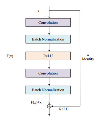
Rolling bear is a major critical component of rotating machinery, as its working condition affects the performance of the equipment. As a result, the condition monitoring and fault diagnosis of bearings get more and more attention. However, the strong background noise makes it difficult to extract the bearing fault features exactly. Furthermore, regular gradient disappearance and overfit appear in traditional network model training. Therefore, taking the printing press bearings as the research object, an intelligent fault diagnosis method based on strong background noise is proposed. This method integrates frequency slice wavelet transform (FSWT), deformable convolution and residual neural network together, and realizes the high-precision fault diagnosis of the printing press bearings. First, FSWT is used to preprocess the original vibration signal to obtain bearing fault features in the time and frequency domain, reconstruct the signal in any frequency band and describe local features accurately. Second, the ResNet is selected as the base network, and the two-dimensional time-frequency diagrams (TFD) obtained by preprocessing are used as input. For the model that has a poor ability to extract subtle features under strong background noise, the deformable convolution layer is introduced to reconstruct the convolution layer of ResNet, called deformable convolution residual neural network (DC-ResNet). Finally, the effectiveness of this method is verified by using the data sets collected under experimental conditions and actual working conditions for fault diagnosis of the printing press. The results show that the DC-ResNet can classify different bearing faults under strong background noise, and the accuracy and stability are greatly improved, which the accuracy meets 93.90%. The intelligent fault diagnosis with high-precision of printing press bearings under complex working conditions is realized by the proposed method.
Citation: Qiumin Wu, Ziqi Zhu, Jiahui Tang, Yukang Xia. Fault diagnosis of printing press bearing based on deformable convolution residual neural network[J]. Networks and Heterogeneous Media, 2023, 18(2): 622-646. doi: 10.3934/nhm.2023027
Rolling bear is a major critical component of rotating machinery, as its working condition affects the performance of the equipment. As a result, the condition monitoring and fault diagnosis of bearings get more and more attention. However, the strong background noise makes it difficult to extract the bearing fault features exactly. Furthermore, regular gradient disappearance and overfit appear in traditional network model training. Therefore, taking the printing press bearings as the research object, an intelligent fault diagnosis method based on strong background noise is proposed. This method integrates frequency slice wavelet transform (FSWT), deformable convolution and residual neural network together, and realizes the high-precision fault diagnosis of the printing press bearings. First, FSWT is used to preprocess the original vibration signal to obtain bearing fault features in the time and frequency domain, reconstruct the signal in any frequency band and describe local features accurately. Second, the ResNet is selected as the base network, and the two-dimensional time-frequency diagrams (TFD) obtained by preprocessing are used as input. For the model that has a poor ability to extract subtle features under strong background noise, the deformable convolution layer is introduced to reconstruct the convolution layer of ResNet, called deformable convolution residual neural network (DC-ResNet). Finally, the effectiveness of this method is verified by using the data sets collected under experimental conditions and actual working conditions for fault diagnosis of the printing press. The results show that the DC-ResNet can classify different bearing faults under strong background noise, and the accuracy and stability are greatly improved, which the accuracy meets 93.90%. The intelligent fault diagnosis with high-precision of printing press bearings under complex working conditions is realized by the proposed method.

| [1] |
J. Jiao, M. Zhao, J. Lin, C. Ding, Deep coupled dense convolution network with complementary data for intelligent fault diagnosis, IEEE Trans. Instrum. Meas., 66 (2019), 9858–9867. https://doi.org/10.1109/tie.2019.2902817 doi: 10.1109/tie.2019.2902817

|
| [2] |
W. Deng, H. Liu, J. Xu, H. Zhao, Y. Song, An improved quantum-inspired differential evolution algorithm for deep belief network, IEEE Trans. Instrum. Meas., 69 (2020), 7319–7327. https://doi.org/10.1109/tim.2020.2983233 doi: 10.1109/tim.2020.2983233
|
| [3] |
J. Liu, A dynamic modelling method of a rotor-roller bearing-housing system with a localized fault including the additional excitation zone, J. Sound Vib., 469 (2020), 115144. https://doi.org/10.1016/j.jsv.2019.115144 doi: 10.1016/j.jsv.2019.115144
|
| [4] |
R. Yan, F. Shen, C. Sun, X. Chen, Knowledge transfer for rotary machine fault diagnosis, IEEE Sens. J., 20 (2019), 8374–8393. https://doi.org/10.1109/jsen.2019.2949057 doi: 10.1109/jsen.2019.2949057
|
| [5] |
Y. Lei, F. Jia, J. Lin, S. Xing, S. Ding, An intelligent fault diagnosis method using unsupervised feature learning towards mechanical big data, IEEE Trans. Ind. Electron., 63 (2016), 3137–3147. https://doi.org/10.1109/tie.2016.2519325 doi: 10.1109/tie.2016.2519325
|
| [6] |
W. Wang, F. Golnaraghi, F. Ismail, Condition monitoring of multistage printing presses, J. Sound Vib., 270 (2004), 755–766. https://doi.org/10.1016/s0022-460x(03)00209-8 doi: 10.1016/s0022-460x(03)00209-8
|
| [7] |
A. Rai, S. Upadhyay, A review on signal processing techniques utilized in the fault diagnosis of rolling element bearings, Tribol. Int., 96 (2016), 289–306. https://doi.org/10.1016/j.triboint.2015.12.037 doi: 10.1016/j.triboint.2015.12.037
|
| [8] |
J. Tang, J. Wu, B. Hu, J. Liu, Towards a fault diagnosis method for rolling bearing with Bi-directional deep belief network, Appl. Acoust., 192 (2022), 1–11. https://doi.org/10.1016/j.apacoust.2022.108727 doi: 10.1016/j.apacoust.2022.108727
|
| [9] |
M. Hmimida, R. Kanawati, Community detection in multiplex networks: A seed-centric approach, Netw. Heterogen. Media, 10 (2015), 71–85. https://doi.org/10.3934/nhm.2015.10.71 doi: 10.3934/nhm.2015.10.71
|
| [10] |
M. Zhao, S. Zhong, X. Fu, B. Tang, P. Michael, Deep residual shrinkage networks for fault diagnosis, IEEE Trans. Industr. Inform., 16 (2019), 4681–4690. https://doi.org/10.1109/tii.2019.2943898 doi: 10.1109/tii.2019.2943898
|
| [11] |
X. Jin, Y. Xu, Research on facial expression recognition based on deep learning, IEEE EITCE, 2019, 1144–1147. https://doi.org/10.1109/eitce47263.2019.9095140 doi: 10.1109/eitce47263.2019.9095140
|
| [12] | R. Wightman, H. Touvron, H. Jégou, Resnet strikes back: An improved training procedure in timm, arXiv, 2021. https://doi.org/10.48550/arXiv.2110.00476 |
| [13] |
Z. Lin, P. Wang, Y. Chen, C. Sun, Fault diagnosis of rolling bearing based on improved convolution neural network, IEEE DDCLS, 2022,643–647. https://doi.org/10.1109/ddcls55054.2022.9858533 doi: 10.1109/ddcls55054.2022.9858533
|
| [14] | S. Zagoruyko, N. Komodakis, Wide residual networks, arXiv, 2016. https://doi.org/10.48550/arXiv.1605.07146 |
| [15] |
I. Konovalenko, P. Maruschak, V. Brevus, Steel surface defect detection using an ensemble of deep Residual neural networks, J. Comput. Inf. Sci. Eng., 22 (2022), 1–7. https://doi.org/10.1115/1.4051435 doi: 10.1115/1.4051435
|
| [16] |
X. Yan, D. She, Y. Xu, Deep order-wavelet convolutional variational autoencoder for fault identification of rolling bearing under fluctuating speed conditions, Expert Syst. Appl., 216 (2022), 119479. https://doi.org/10.1016/j.eswa.2022.119479 doi: 10.1016/j.eswa.2022.119479
|
| [17] |
B. Peng, H. Xia, X. Lv, M. Annor-Nyarko, S. Zhu, Y. Liu, et al., An intelligent fault diagnosis method for rotating machinery based on data fusion and deep Residual neural network, Appl. Intell., 52 (2022), 3051–3065. https://doi.org/10.1007/s10489-021-02555-4 doi: 10.1007/s10489-021-02555-4
|
| [18] |
X. Yan, D. She, Y. Xu, J. Ping, Deep regularized variational autoencoder for intelligent fault diagnosis of rotor–bearing system within entire life-cycle process, Knowledge-Based Syst., 226 (2021), 107142. https://doi.org/10.1016/10.1016/j.knosys.2021.107142 doi: 10.1016/10.1016/j.knosys.2021.107142
|
| [19] |
B. Wang, Y. Lei, N. Li, T. Yan, Deep separable convolution network for remaining useful life prediction of machinery, Mech. Syst. Signal Process., 134 (2019), 106330. https://doi.org/10.1016/j.ymssp.2019.106330 doi: 10.1016/j.ymssp.2019.106330
|
| [20] |
P. Liang, W. Wang, X. Yuan, S. Liu, L. Zhang, Y. Cheng, Intelligent fault diagnosis of rolling bearing based on wavelet transform and improved Residual neural network under noisy labels and environment, Eng. Appl. Artif. Intell., 115 (2022), 105269. https://doi.org/10.1016/j.engappai.2022.105269 doi: 10.1016/j.engappai.2022.105269
|
| [21] |
W. Zhang, Z. Wang, X. Li, Blockchain-based decentralized federated transfer learning methodology for collaborative machinery fault diagnosis, Reliab. Eng. Syst. Safe., 229 (2023), 108885. https://doi.org/10.1016/j.ress.2022.108885 doi: 10.1016/j.ress.2022.108885
|
| [22] |
X. Yan, Y. Liu, M. Jia, Multiscale cascading deep belief network for fault identification of rotating machinery under various working conditions, Knowledge-Based Syst., 193 (2020), 105484. https://doi.org/10.1016/j.knosys.2020.105484 doi: 10.1016/j.knosys.2020.105484
|
| [23] |
P. Lin, Z. Qian, X. Lu, Y. Lin, Y. Lai, S. Cheng, Compound fault diagnosis model for Photovoltaic array using multi-scale SE-Residual neural network, Sustain. Energy. Technol., 50 (2022), 101785. https://doi.org/10.1016/j.seta.2021.101785 doi: 10.1016/j.seta.2021.101785
|
| [24] |
L. Wan, Y. Li, K. Chen, K. Gong, C. Li, A novel deep convolution multi-adversarial domain adaptation model for rolling bearing fault diagnosis, Measurement, 191 (2022), 110752. https://doi.org/10.1016/j.measurement.2022.110752 doi: 10.1016/j.measurement.2022.110752
|
| [25] |
X. Yan, Y. Liu, Y. Xu, M. Jia, Multistep forecasting for diurnal wind speed based on hybrid deep learning model with improved singular spectrum decomposition, Energy Convers. Manage., 225 (2020), 113456. https://doi.org/10.1016/j.enconman.2020.113456 doi: 10.1016/j.enconman.2020.113456
|
| [26] |
P. Yang, Q. Liu, B. Wang, W. Li, Z. Li, M. Sun, An empirical study of fault diagnosis methods of a dissolved oxygen sensor based on ResNet-50, Int. J. Sens. Netw., 39 (2022), 205–214. https://doi.org/10.1504/ijsnet.2022.124566 doi: 10.1504/ijsnet.2022.124566
|
| [27] |
X. Hao, Y. Zheng, L. Lu, H. Pan, Research on intelligent fault diagnosis of rolling bearing based on improved deep residual neural network, Appl. Sci., 11 (2021), 10889. https://doi.org/10.3390/app112210889 doi: 10.3390/app112210889
|
| [28] |
K. Zhang, B. Tang, L. Deng, X. Liu, A hybrid attention improved Residual neural network based fault diagnosis method of wind turbines gearbox, Measurement, 179 (2021), 109491. https://doi.org/10.1016/j.measurement.2021.109491 doi: 10.1016/j.measurement.2021.109491
|
| [29] |
Y. Wang, J. Liang, X. Gu, D. Ling, H. Yu, Multi-scale attention mechanism Residual neural network for fault diagnosis of rolling bearings, Proc. Inst. Mech. Eng., Part C: J. Mech. Eng. Sci., 236 (2022), 10615–10629. https://doi.org/10.1177/09544062221104598 doi: 10.1177/09544062221104598
|
| [30] |
Z. Lai, X. Zhu, J. Wu, Generative focused feedback Residual neural networks for image steganalysis and hidden information reconstruction, Appl. Soft. Comput., 129 (2022), 109550. https://doi.org/10.1016/j.asoc.2022.109550 doi: 10.1016/j.asoc.2022.109550
|
| [31] |
D. Hartono, D. Halim, G. W. Roberts, Gear fault diagnosis using an improved reassigned smoothed Pseudo Wigner-Ville distribution, Cogent Eng., 5 (2018), 1436928. https://doi.org/10.1080/23311916.2018.1436928 doi: 10.1080/23311916.2018.1436928
|
| [32] |
S. Chegini, A. Bagheri, F. Najafi, A new intelligent fault diagnosis method for bearing in different speeds based on the FDAF-score algorithm, binary particle swarm optimization, and support vector machine, Soft. Comput., 24 (2020), 10005–10023. https://doi.org/10.1007/s00500-019-04516-z doi: 10.1007/s00500-019-04516-z
|
| [33] |
K. V. Surti, C. A. Naik, Bearing condition monitoring of induction motor based on discrete wavelet transform & k-nearest neighbor, IEEE I2CT, 2018, 1–5. https://doi.org/10.1109/i2ct.2018.8529687 doi: 10.1109/i2ct.2018.8529687
|
| [34] |
X. Li, Y. Xu, N. Li, B. Yang, Y. Lei, Remaining useful life prediction with partial sensor malfunctions using deep adversarial networks, IEEE/CAA J. Autom. Sinica., 10 (2022), 121–134. https://doi.org/10.1109/jas.2022.105935 doi: 10.1109/jas.2022.105935
|
| [35] |
R. Dubey, D. Agrawal, Bearing fault classification using ANN-based Hilbert footprint analysis, Iet. Scl. Meas. Technol., 9 (2015), 1016–1022. https://doi.org/10.1049/iet-smt.2015.0026 doi: 10.1049/iet-smt.2015.0026
|
| [36] |
J. Tian, C. Morillo, M. H. Azarian, M. Pecht, Motor bearing fault detection using spectral kurtosis-based feature extraction coupled with K-nearest neighbor distance analysis, Ieee. T. Ind. Electron., 63 (2015), 1793-1803. https://doi.org/10.1109/tie.2015.2509913 doi: 10.1109/tie.2015.2509913
|
| [37] |
M. Amar, I. Gondal, C. Wilson, Vibration spectrum imaging: A novel bearing fault classification approach, IEEE Trans. Ind. Electron., 62 (2014), 494–502. https://doi.org/10.1109/tie.2014.2327555 doi: 10.1109/tie.2014.2327555
|
| [38] |
W. Zhang, Y. Ding, X. Yan, M. Jia, Weak multiple fault detection based on weighted morlet wavelet-overlapping group sparse for rolling bearing fault diagnosis, Appl. Sci., 10 (2020), 2057. https://doi.org/10.3390/app10062057 doi: 10.3390/app10062057
|
| [39] |
W. Mao, L. He, Y. Yan, J. Wang, Online sequential prediction of bearings imbalanced fault diagnosis by extreme learning machine, Mech. Syst. Signal. Pr., 83 (2017), 450–473. https://doi.org/10.1016/j.ymssp.2016.06.024 doi: 10.1016/j.ymssp.2016.06.024
|
| [40] |
H. Zhao, M. Liu, Y. Sun, Z. Chen, G. Duan, X. Cao, Fault diagnosis of control moment gyroscope based on a new CNN scheme using attention-enhanced convolution block, Sci. China Technol. Sci., 65 (2022), 2605–2616. https://doi.org/10.1007/S11431-022-2141-9 doi: 10.1007/S11431-022-2141-9
|
| [41] |
C. Duan, Q. Gao, X. Xu, Generator unit fault diagnosis using the frequency slice wavelet transform time-frequency analysis method, Proc. CSEE, 33 (2013), 96–103. https://doi.org/10.13334/j.0258-8013.pcsee.2013.32.014 doi: 10.13334/j.0258-8013.pcsee.2013.32.014
|
| [42] |
Z. Sheng, Y. Xu, K. Zhang, Applications in bearing fault diagnosis of an improved Kurtogram algorithm based on flexible frequency slice wavelet transform filter bank, Measurement, 174 (2021), 108975. https://doi.org/10.1016/j.measurement.2021.108975 doi: 10.1016/j.measurement.2021.108975
|
| [43] | X. Zhong, Research on time-frequency analysis methods and its applications to rotating machinery fault diagnosis, PhD dissertation, Wuhan University of Science and Technology, Wuhan, 2014. |
| [44] |
K. Hirasawa, M Ohbayashi, M Koga, M Harada, Forward propagation universal learning network, IEEE ICNN'96, 1 (1996), 353–358. https://doi.org/10.1109/icnn.1996.548917 doi: 10.1109/icnn.1996.548917
|
| [45] |
F. Chen, F. Wu, J. Xu, G. Gao, Q Ge, X. Jing, Adaptive Deformable Convolutional Network, Neurocomputing, 453 (2021), 853–864. https://doi.org/10.1016/j.neucom.2020.06.128 doi: 10.1016/j.neucom.2020.06.128
|
| [46] |
W. Smith, R. Randall, Rolling element bearing diagnostics using the Case Western Reserve University data: A benchmark study, Mech. Syst. Signal. Pr., 64 (2015), 100–131. https://doi.org/10.1016/j.ymssp.2015.04.021 doi: 10.1016/j.ymssp.2015.04.021
|
| [47] |
O. Caelen, A Bayesian interpretation of the confusion matrix, Ann. Math. Artif. Intel., 81 (2017), 429–450. https://doi.org/10.1007/s10472-017-9564-8 doi: 10.1007/s10472-017-9564-8
|
| [48] |
W. Lu, X. Yan, Visualizing high-dimensional industrial process based on deep reinforced discriminant features and a stacked supervised t-distributed stochastic neighbor embedding network, Expert Syst. Appl., 186 (2021), 115389. https://doi.org/10.1016/j.eswa.2021.115389 doi: 10.1016/j.eswa.2021.115389
|
| [49] |
R. Selvaraju, M. Cogswell, A. Das, R. Vedantam, D. Parikh, D, Batra Grad-cam: Visual explanations from deep networks via gradient-based localization, Proc. IEEE Int. Conf. Comput. Vis., 128 (2020), 336–359. https://doi.org/10.1007/s11263-019-01228-7 doi: 10.1007/s11263-019-01228-7
|


Figures(18) / Tables(7)
Qiumin Wu, Ziqi Zhu, Jiahui Tang, Yukang Xia. Fault diagnosis of printing press bearing based on deformable convolution residual neural network[J]. Networks and Heterogeneous Media, 2023, 18(2): 622-646. doi: 10.3934/nhm.2023027


 DownLoad: