Structure-preserving scheme for one dimension and two dimension fractional KGS equations

Junjie Wang; Yaping Zhang; Liangliang Zhai; Junjie Wang; Yaping Zhang; Liangliang Zhai

doi:10.3934/nhm.2023019

Networks and Heterogeneous Media

2023, Volume 18, Issue 1: 463-493. doi: 10.3934/nhm.2023019

Previous Article Next Article

Research article Special Issues

Structure-preserving scheme for one dimension and two dimension fractional KGS equations

1.
School of Mathematics and Statistical, Pu'er University, Yunnan, 665000, China
2.
School of Science, Shaoyang University, Hunan, 422000, China
3.
School of Science, Xi'an Shiyou University, Shaanxi, 710065, China

Received: 30 October 2022 Revised: 07 December 2022 Accepted: 21 December 2022 Published: 13 January 2023

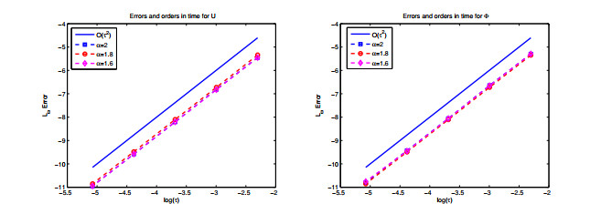
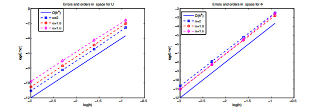
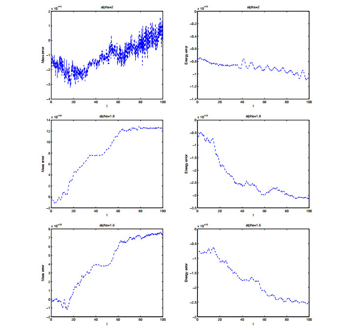
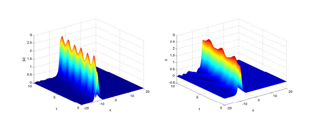
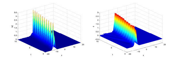
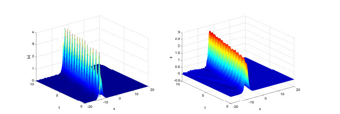
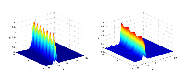
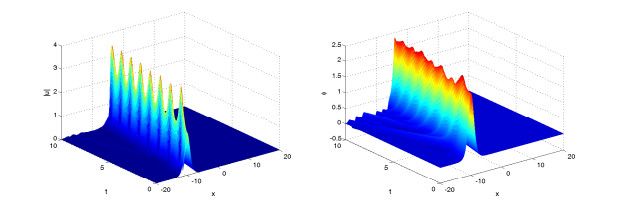
In the paper, we study structure-preserving scheme to solve general fractional Klein-Gordon-Schrödinger equations, including one dimension case and two dimension case. First, the high central difference scheme and Crank-Nicolson scheme are used to one dimension fractional Klein-Gordon-Schrödinger equations. We show that the arising scheme is uniquely solvable, and approximate solutions converge to the exact solution at the rate $ O(\tau^2+h^4) $. Moreover, we prove that the resulting scheme can preserve the mass and energy conservation laws. Second, we show Crank-Nicolson scheme for two dimension fractional Klein-Gordon-Schrödinger equations, and the proposed scheme preserves the mass and energy conservation laws in discrete formulations. However, the obtained discrete system is nonlinear system. Then, we show a equivalent form of fractional Klein-Gordon-Schrödinger equations by introducing some new auxiliary variables. The new system is discretized by the high central difference scheme and scalar auxiliary variable scheme, and a linear discrete system is obtained, which can preserve the energy conservation law. Finally, the numerical experiments including one dimension and two dimension fractional Klein-Gordon-Schrödinger systems are given to verify the correctness of theoretical results.
- Fractional Klein-Gordon-Schrödinger equations,
- conservation law,
- convergence,
- high central difference scheme,
- scalar auxiliary variable scheme
Citation: Junjie Wang, Yaping Zhang, Liangliang Zhai. Structure-preserving scheme for one dimension and two dimension fractional KGS equations[J]. Networks and Heterogeneous Media, 2023, 18(1): 463-493. doi: 10.3934/nhm.2023019

Related Papers:

Abstract

In the paper, we study structure-preserving scheme to solve general fractional Klein-Gordon-Schrödinger equations, including one dimension case and two dimension case. First, the high central difference scheme and Crank-Nicolson scheme are used to one dimension fractional Klein-Gordon-Schrödinger equations. We show that the arising scheme is uniquely solvable, and approximate solutions converge to the exact solution at the rate $ O(\tau^2+h^4) $. Moreover, we prove that the resulting scheme can preserve the mass and energy conservation laws. Second, we show Crank-Nicolson scheme for two dimension fractional Klein-Gordon-Schrödinger equations, and the proposed scheme preserves the mass and energy conservation laws in discrete formulations. However, the obtained discrete system is nonlinear system. Then, we show a equivalent form of fractional Klein-Gordon-Schrödinger equations by introducing some new auxiliary variables. The new system is discretized by the high central difference scheme and scalar auxiliary variable scheme, and a linear discrete system is obtained, which can preserve the energy conservation law. Finally, the numerical experiments including one dimension and two dimension fractional Klein-Gordon-Schrödinger systems are given to verify the correctness of theoretical results.

References

[1]	B. Guo, K. Pu, F. Huang, Fractional Partial Differential Equations and their Numerical Solutions, Singapore: World Scientific, 2011.
[2]	Z. Sun, G. Gao, Finite Difference Methods for Fractional-order Differential Equations, Beijing: Science Press, 2015.
[3]	F. Liu, P. Zhuang, Q. Liu, Numerical Methods and Their Applications of Fractional Partial Differential Equations, Beijing: Science Press, 2015.
[4]	C. Pozrikidis, The fractional Laplacian, Baco Raton: CRC Press, 2016.
[5]	J. Xia, S. Han, M. Wang, The exact solitary wave solution for the Klein-Gordon-Schrödinger equations, Appl. Math. Mech., 23 (2002), 52–58. https://doi.org/10.1007/BF02437730 doi: 10.1007/BF02437730
[6]	B. Guo, Y. Li, Attractor for dissipative Klein-Gordon-Schrödinger equations in $R^3$, J Differ Equ, 136 (1997), 356–377.
[7]	H. Pecher, Global solutions of the Klein-Gordon-Schrödinger system with rough data, Differ. Integral Equ., 17 (2004), 179–214. https://doi.org/10.2752/089279304786991837 doi: 10.2752/089279304786991837
[8]	L. Zhang, Convergence of a conservative difference scheme for a class of Klein-Gordon-Schrödinger equations in one space dimension, Appl Math Comput, 163 (2005), 343–355. https://doi.org/10.1016/j.amc.2004.02.010 doi: 10.1016/j.amc.2004.02.010
[9]	J. Hong, S. Jiang, C. Li, Explicit multi-symplectic methods for Klein-Gordon-Schrödinger equations, J. Comput. Phys., 228 (2009), 3517–3532. https://doi.org/10.1016/j.jcp.2009.02.006 doi: 10.1016/j.jcp.2009.02.006
[10]	T. Wang, Optimal point-wise error estimate of a compact difference scheme for the Klein-Gordon-Schrödinger equation, J. Math. Anal. Appl., 412 (2014), 155–167. https://doi.org/10.1016/j.jmaa.2013.10.038 doi: 10.1016/j.jmaa.2013.10.038
[11]	W. Bao, L. Yang, Efficient and accurate numerical methods for the Klein-Gordon-Schrödinger equations, J. Comput. Phys., 225 (2007), 1863–1893. https://doi.org/10.1016/j.jcp.2007.02.018 doi: 10.1016/j.jcp.2007.02.018
[12]	L. Kong, J. Zhang, Y. Cao, Y. Duan, H. Huang, Semi-explicit symplectic partitioned Runge-Kutta Fourier pseudo-spectral scheme for Klein-Gordon-Schrödinger equations, Commun Comput Phys, 181 (2010), 1369–1377.
[13]	C. Huang, G. Guo, D. Huang, Q. Li, Global well-posedness of the fractional Klein-Gordon-Schrödinger system with rough initial data, Sci. China Math., 59 (2016), 1345–1366. https://doi.org/10.1007/s11425-016-5133-6 doi: 10.1007/s11425-016-5133-6
[14]	J. Wang, A. Xiao, An efficient conservative difference scheme for fractional Klein-Gordon-Schrödinger equations, Appl Math Comput, 320 (2018), 691–709. https://doi.org/10.1016/j.amc.2017.08.035 doi: 10.1016/j.amc.2017.08.035
[15]	J. Wang, A. Xiao, C. Wang, A conservative difference scheme for space fractional Klein-Gordon-Schrödinger equations with a High-Degree Yukawa Interaction, East Asian J Applied Math, 8 (2018), 715–745.
[16]	J. Wang, A. Xiao, Conservative Fourier spectral method and numerical investigation of space fractional Klein-Gordon-Schrödinger equations, Appl Math Comput, 350 (2019), 348–365. https://doi.org/10.1016/j.amc.2018.12.046 doi: 10.1016/j.amc.2018.12.046
[17]	J. Wang, Symplectic-preserving Fourier spectral scheme for space fractional Klein-Gordon-Schrödinger equations, Numer Methods Partial Differ Equ, 37 (2021), 1030–1056. https://doi.org/10.1002/num.22565 doi: 10.1002/num.22565
[18]	P. Wang, C. Huang, L. Zhao, Point-wise error estimate of a conservative difference scheme for the fractional Schrödinger equation, J. Comput. Appl. Math., 306 (2016), 231–247. https://doi.org/10.1016/j.cam.2016.04.017 doi: 10.1016/j.cam.2016.04.017
[19]	X. Zhao, Z. Sun, Z. Hao, A fourth-order compact ADI scheme for two-dimensional nonlinear space fractional Schrödinger equation, SIAM J Sci Comput, 36 (2014), A2865–A2886. https://doi.org/10.1137/140961560 doi: 10.1137/140961560
[20]	A. Xiao, J. Wang, Symplectic scheme for the Schrödinger equation with fractional Laplacian, Appl Numer Math, 146 (2019), 469–487. https://doi.org/10.1016/j.apnum.2019.08.002 doi: 10.1016/j.apnum.2019.08.002
[21]	J. Wang, High-order conservative schemes for the space fractional nonlinear Schrödinger equation, Appl Numer Math, 165 (2021), 248–269. https://doi.org/10.1016/j.apnum.2021.02.017 doi: 10.1016/j.apnum.2021.02.017
[22]	L. Zhai, J. Wang, High-order conservative scheme for the coupled space fractional nonlinear Schrödinger equations, Int. J. Comput. Math., 99 (2022), 607–628. https://doi.org/10.1080/00207160.2021.1925889 doi: 10.1080/00207160.2021.1925889
[23]	M. ortigueira, Riesz potential operators and inverses via fractional centred derivatives, Int J Math Math Sci, 2006 (2006), 1–12.
[24]	J. Cui, Z. Sun, H. Wu, A high accurate and conservative difference scheme for the solution of nonlinear schrödinger equation, Numer Math J Chin Univ, 37 (2015), 31–52.
[25]	K. Kirkpatrick, E. Lenzmann, G. Staffilani, On the continuum limit for discrete NLS with long-range lattice interactions, Commun. Math. Phys., 317 (2013), 563–591. https://doi.org/10.1007/s00220-012-1621-x doi: 10.1007/s00220-012-1621-x
[26]	D. Hu, W. Cai, Y. Fu, Y. Wang, Fast dissipation-preserving difference scheme for nonlinear generalized wave equations with the integral fractional Laplacian, Commun Nonlinear Sci Numer Simul, 99 (2021), 105786.
[27]	Z. Hao, Z. Zhang, R. Du, Fractional centered difference scheme for high-dimensional integral fractional Laplacian, J. Comput. Phys., 424 (2021), 109851. https://doi.org/10.1016/j.jcp.2020.109851 doi: 10.1016/j.jcp.2020.109851

Reader Comments

Your name:*

Email:*
© 2023 the Author(s), licensee AIMS Press. This is an open access article distributed under the terms of the Creative Commons Attribution License (http://creativecommons.org/licenses/by/4.0)