We propose a time-delayed Cucker-Smale type model(CS model), which can be applied to modeling (1) collective dynamics of self-propelling agents and (2) the dynamical system of stock return volatility in a financial market. For both models, we assume that it takes a certain amount of time to collect/process information about the current position/return configuration until velocity/volatility adjustment is made. We provide a sufficient condition under which flocking phenomena occur. We also identify the initial configuration for a two-agent case, in which collective behaviors are accelerated by changes in the delay parameter. Numerical illustrations and financial simulations are carried out to verify the validity of the model.
Citation: Hyeong-Ohk Bae, Seung Yeon Cho, Jane Yoo, Seok-Bae Yun. Effect of time delay on flocking dynamics[J]. Networks and Heterogeneous Media, 2022, 17(5): 803-825. doi: 10.3934/nhm.2022027
We propose a time-delayed Cucker-Smale type model(CS model), which can be applied to modeling (1) collective dynamics of self-propelling agents and (2) the dynamical system of stock return volatility in a financial market. For both models, we assume that it takes a certain amount of time to collect/process information about the current position/return configuration until velocity/volatility adjustment is made. We provide a sufficient condition under which flocking phenomena occur. We also identify the initial configuration for a two-agent case, in which collective behaviors are accelerated by changes in the delay parameter. Numerical illustrations and financial simulations are carried out to verify the validity of the model.

| [1] | The Kuramoto model: A simple paradigm for synchronization phenomena. Rev. Mod. Phys. (2005) 77: 137. |
| [2] |
Application of flocking mechanism to the modeling of stochastic volatility. Math. Models Methods Appl. Sci. (2013) 23: 1603-1628. 
|
| [3] |
Vehicular traffic, crowds and swarms: From kinetic theory and multiscale methods to applications and research perspectives. Math. Mod. Meth. Appl. Sci. (2019) 29: 1901-2005.
|
| [4] |
Modeling of self-organized systems interacting with a few individuals: From microscopic to macroscopic dynamics. Appl. Math. Lett. (2013) 26: 397-401.
|
| [5] | Stochastic autoregressive volatility: A framework for volatility modeling. Math. Fin. (1994) 42: 75-102. |
| [6] |
A kinetic description for the herding behavior in financial market. J. Stat Phys. (2019) 176: 398-424.
|
| [7] |
A particle model for the herding phenomena induced by dynamic market signals. J. Stat. Phys. (2019) 177: 365-398.
|
| [8] |
H.-O. Bae, S.-Y. Ha, M. Kang, Y. Kim, H. Lim and J. Yoo, Time-delayed stochastic volatility model, Phys. D: Nonlinear Phen., 430 (2022), 133088, 14 pp. |
| [9] |
Emergent dynamics of the first-order stochastic Cucker-Smale model and application to finance. Math. Methods Appl. Sci. (2019) 42: 6029-6048.
|
| [10] |
A mathematical model for volatility flocking with a regime switching mechanism in a stock market. Math. Models Methods Appl. Sci. (2015) 25: 1299-1335.
|
| [11] | Volatility flocking by cucker-smale mechanism in financial markets. Asia-Pacific Fin. Mkts. (2020) 27: 387-414. |
| [12] |
Fractionally integrated generalized autoregressive conditional heteroskedasticity. J. Econom. (1996) 74: 3-30.
|
| [13] |
Mathematics and complexity in life and human sciences. Math. Mod. Meth. Appl. Sci. (2010) 20: 1391-1395.
|
| [14] |
On the correlation structure of the generalize autoregressive conditional heteroscedastic process. J. Time. Ser. Anal. (1988) 9: 121-131.
|
| [15] |
Common persistence in conditional variances. Econometrica (1993) 61: 167-186.
|
| [16] | A capital asset pricing model with time-varying covariances. J. Pol. Econ. (1988) 96: 116-131. |
| [17] |
Sharp conditions to avoid collisions in singular Cucker-Smale interactions. Nonlinear Anal. Real World Appl. (2017) 37: 317-328.
|
| [18] |
Cucker-Smale model with normalized communication weights and time delay. Kinet. Relat. Models (2017) 10: 1011-1033.
|
| [19] |
Emergent behavior of Cucker-Smale model with normalized weights and distributed time delays. Netw. Heterog. Media (2019) 14: 789-804.
|
| [20] |
Emergent behavior in flocks. IEEE Trans. Automat. Control (2007) 52: 852-862.
|
| [21] | Modifications of the optimal velocity traffic model to include delay due to driver reaction time. Phys. A: Stat. Mech. and its Appl. (2003) 319: 557-567. |
| [22] |
Interplay of time-delay and velocity alignment in the Cucker-Smale model on a general digraph. Discrete Contin. Dyn. Syst. Ser. B (2019) 24: 5569-5596.
|
| [23] |
Time-delay effect on the flocking in an ensemble of thermomechanical Cucker-Smale particles. J. Differential Equations (2019) 266: 2373-2407.
|
| [24] | Self-propelled particles with soft-core interactions: Patterns, stability, and collapse. Phys. Rev. Lett. (2006) 96: 104302. |
| [25] |
Autoregressive conditional heteroskedasticity with estimates of the variance of United Kingdom inflation. Econometrica (1982) 50: 987-1007.
|
| [26] |
From individual choice to group decision-making. Phys A: Stat. Mech. and its Appl. (2000) 287: 644-659.
|
| [27] |
Nonlocality of reaction-diffusion equations induced by delay: Biological modeling and nonlinear dynamics. J. Math. Sci. (2004) 124: 5119-5153.
|
| [28] | Emergence of time-asymptotic flocking in a stochastic Cucker-Smale system. Commun. Math. Sci. (2009) 7: 453-469. |
| [29] |
Synchronization of Kuramoto oscillators with adaptive couplings. SIAM J. Appl. Dyn. Syst. (2016) 15: 162-194.
|
| [30] | Unobserved component time series models with ARCH disturbances. J. Econom. (1992) 52: 129-157. |
| [31] | A multivariate GARCH model of international transmission of stock returns and volatility: The case of United States and Canada. J. Bus. Econ. Stat. (1995) 13: 11-25. |
| [32] | A continuous-time Garch model for stochastic volatility with delay. Can. Appl. Math. Q. (2005) 13: 123-149. |
| [33] |
On the use of delay equations in engineering applications. J. Vib. Cont. (2010) 16: 943-960.
|
| [34] |
Global stability of a biological model with time delay. Proc. Amer. Math. Soc. (1986) 96: 75-78.
|
| [35] |
Cucker-Smale flocking under rooted leadership with fixed and switching topologies. SIAM J. Appl. Math. (2010) 70: 3156-3174.
|
| [36] | Consensus over directed static networks with arbitrary finite communication delays. Phys. Rev. E. (2009) 80: 066121. |
| [37] |
Kalman filtering for multiple time-delay systems. Automatica (2005) 41: 1455-1461.
|
| [38] |
Predator-prey models with delay and prey harvesting. J. Math. Biol. (2001) 43: 247-267.
|
| [39] |
A new model for self-organized dynamics and its flocking behavior. J. Stat. Phys. (2011) 144: 923-947.
|
| [40] |
Cucker-Smale flocking with inter-particle bonding forces. IEEE Trans. Automat. Cont. (2010) 55: 2617-2623.
|
| [41] | The use of delay differential equations in chemical kinetics. J. Phys. Chem. (1996) 100: 8323-8330. |
| [42] |
Cucker-Smale flocking under hierarchical leadership. SIAM J. Appl. Math. (2007/08) 68: 694-719.
|
| [43] |
Stability of traffic flow behavior with distributed delays modeling the memory effects of the drivers. SIAM J. Appl. Math. (2008) 68: 738-759.
|
| [44] |
A simple chaotic delay differential equation. Phys. Lett. A. (2007) 366: 397-402.
|
| [45] |
A stochastic delay financial model. Proc. Amer. Math. Soc. (2005) 133: 1837-1841.
|
| [46] |
Novel type of phase transition in a system of self-driven particles. Phys. Rev. Lett. (1995) 75: 1226-1229.
|
| [47] |
On equilibria and consensus of the Lohe model with identical oscillators. SIAM J. Appl. Dyn. Syst. (2018) 17: 1716-1741.
|
Figures(7)
Hyeong-Ohk Bae, Seung Yeon Cho, Jane Yoo, Seok-Bae Yun. Effect of time delay on flocking dynamics[J]. Networks and Heterogeneous Media, 2022, 17(5): 803-825. doi: 10.3934/nhm.2022027

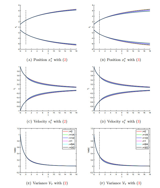
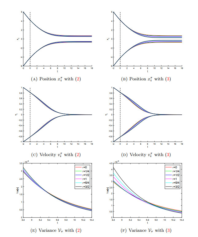
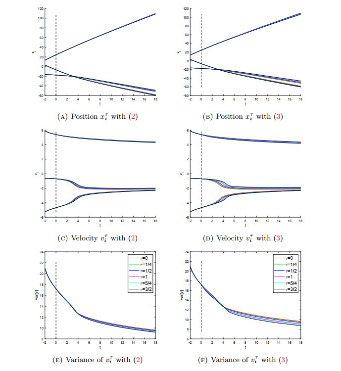
Verification of Theorem 3.3: Time evolution of position(top), velcocity(middle) and variance(bottom) with two types of communication (2)(left) and (3)(right). Each line show the results with various time delays. History data and other parameter values are given in Section 5.1.1
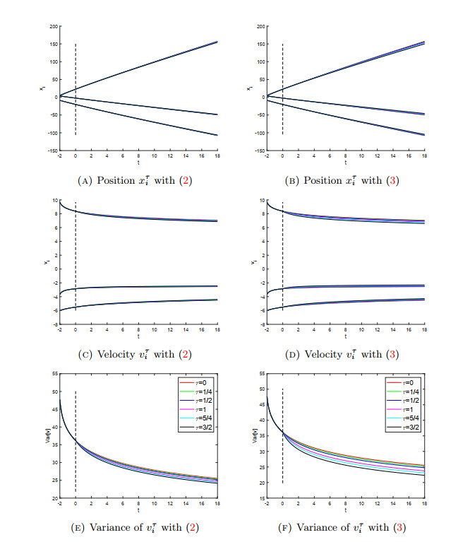
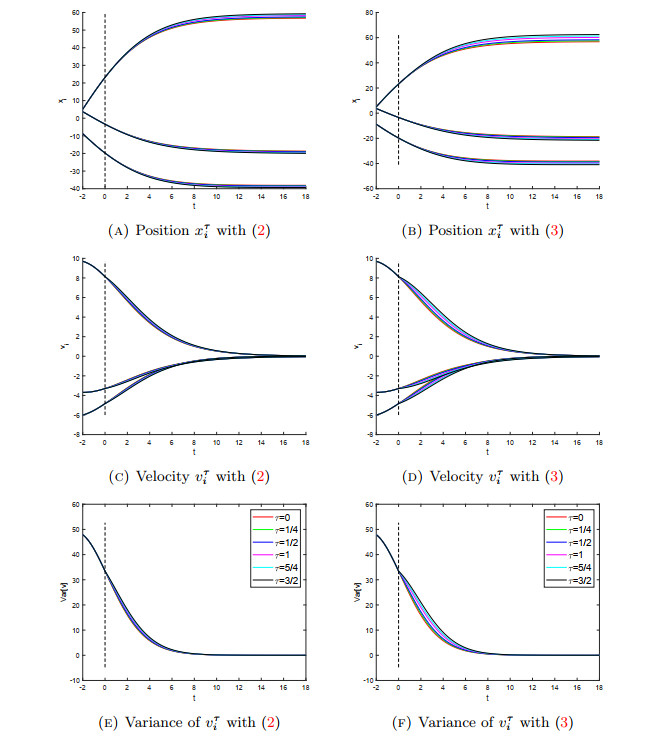
Violation of condition (6): Time evolution of position(top), velcocity(middle) and variance(bottom) with two types of communication (2)(left) and (3)(right). Each line show the results with various time delays. History data and other parameter values are given in Section 5.1.2
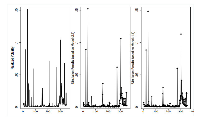
Simulation Results for
Simulation Results with
Simulation Results with
Comparison of real and simulated volatility data of General Electric (GE)
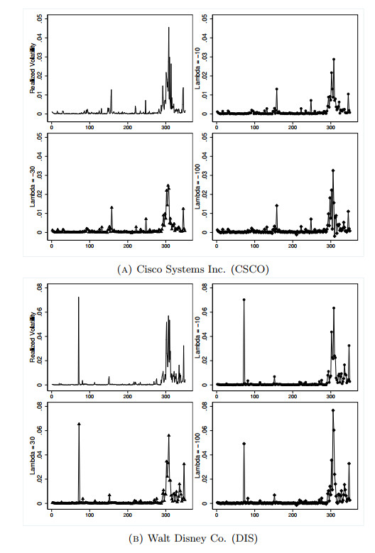
Historical and Simulated Volatilities with different


 DownLoad: