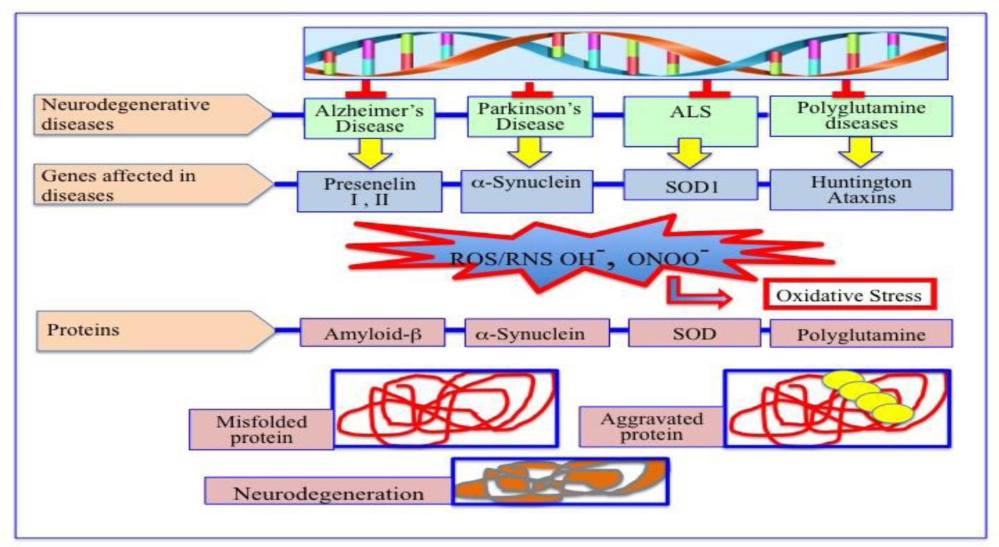
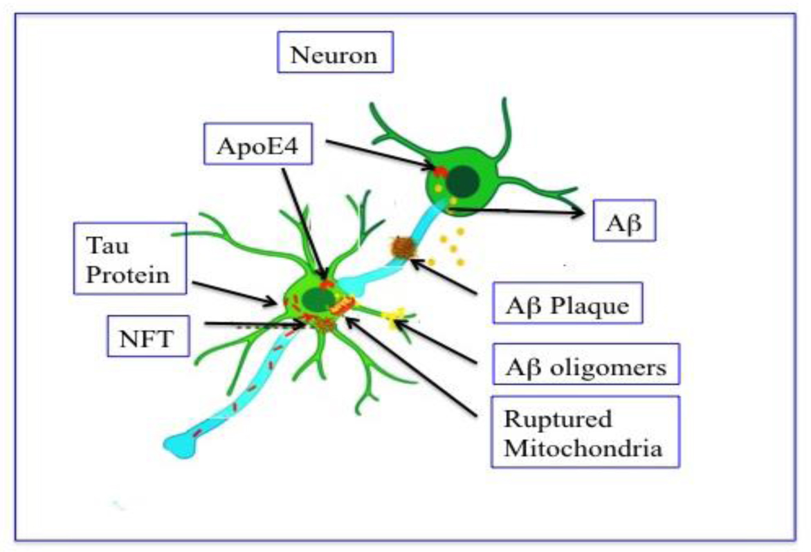
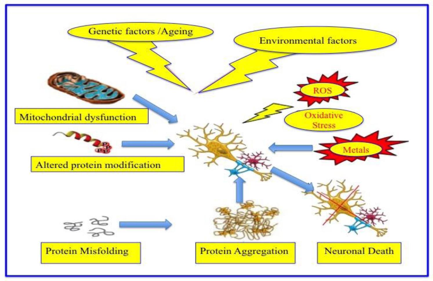
Degenerative nerve diseases affect body's balance, movement, speech, breathing and heart function. Classification of neurodegenerative disorders can be done on the basis of their molecular cause, like abnormal protein aggregation, involved cell death or loss of function of involved cell. Parkinson's disease (PD) is associated with aggregation of α-synuclein, while Alzheimer disease (AD) is associated with tau, amyloid-β42 protein aggregation. TDP-43 aggregation was found in Amyloidosis. Besides, Argyrophilic grain disease (AGD); Amyotrophic lateral sclerosis (ALS); Astrocyte plaque (AP); ALS and Parkinsonism-Dementia Complex (APDC); Aging-related tau astrogliopathy (ARTAG); Ballooned neuron (BN); Cerebral age-related TDP-43 with sclerosis (CARTS); Corticobasal degeneration (CBD); Chronic traumatic encephalopathy (CTE); Dementia with Lewy bodies (DLB); Dystrophic neuritis (DN); Facial onset sensory and motor neuronopathy (FOSMN); Glial cytoplasmic inclusions (GCI); globular glial tauopathy (GGT); Guadeloupean Parkinsonism (GP); idiopathic REM sleep behavior disorder (iRBD); Limbic-predominant age-related TDP-43 encephalopathy (LATE); Lewy bodies (LB); Lewy body diseases (LBD); Lewy neuritis (LN); muscle cells (MC); multiple system atrophy (MSA); multisystem proteinopathy (MSP); Neuronal cytoplasmic inclusions (NCI); neurofibrillary tangles (NFT); neuronal intranuclear inclusions (NII); neuropil threads (NPT); Nodding Syndrome (NS); oligodendroglial coiled bodies (OCB); oligodendroglial Pick's body-like inclusions (OPiBLI); pure autonomic failure (PAF); primary age-related tauopathy (PART); Pick's bodies (PiB); Pick's disease (PiD); Primary lateral sclerosis (PLS); Progressive muscular atrophy (PMA); progressive supranuclear palsy (PSP); pretangles (PT); tufted astrocyte (TA), are several neurodegenerative diseases name according to their involved protein factor(s).
The cause may be genetic, may also be sporadic. Alcoholism, pesticides, a tumor, or a stroke are sometimes noticed in the disease background. Sometimes the cause remains totally unknown. Neurodegeneration, till date, cannot be cured. Only some palliative treatments may relieve some of the symptoms but temporarily. Further, some types of NDD could also be fatal.
Our focus, in this review, is mainly on AD and PD since they vastly affect millions of people in the world, and occurs when nerve cells lose functional ability and/or die over time. AD and PD, the likelihood of developing the issues rise dramatically with age. Unfortunately, there is no cure at present for them except some palliative measure to give some comfort to the victims. Improvement of our understanding about the cause(s) of neurodegenerative diseases may help to design the new approaches for treatment and prevention of the ailments. In recent days, high-throughput technologies like RNA sequencing, network biology, and Omics data provide insights of all neurodegenerative disease.
Citation: Ashok Chakraborty, Anil Diwan. Molecular mechanisms of neurodegenerative disease (NDD)[J]. AIMS Molecular Science, 2023, 10(3): 171-185. doi: 10.3934/molsci.2023012
Degenerative nerve diseases affect body's balance, movement, speech, breathing and heart function. Classification of neurodegenerative disorders can be done on the basis of their molecular cause, like abnormal protein aggregation, involved cell death or loss of function of involved cell. Parkinson's disease (PD) is associated with aggregation of α-synuclein, while Alzheimer disease (AD) is associated with tau, amyloid-β42 protein aggregation. TDP-43 aggregation was found in Amyloidosis. Besides, Argyrophilic grain disease (AGD); Amyotrophic lateral sclerosis (ALS); Astrocyte plaque (AP); ALS and Parkinsonism-Dementia Complex (APDC); Aging-related tau astrogliopathy (ARTAG); Ballooned neuron (BN); Cerebral age-related TDP-43 with sclerosis (CARTS); Corticobasal degeneration (CBD); Chronic traumatic encephalopathy (CTE); Dementia with Lewy bodies (DLB); Dystrophic neuritis (DN); Facial onset sensory and motor neuronopathy (FOSMN); Glial cytoplasmic inclusions (GCI); globular glial tauopathy (GGT); Guadeloupean Parkinsonism (GP); idiopathic REM sleep behavior disorder (iRBD); Limbic-predominant age-related TDP-43 encephalopathy (LATE); Lewy bodies (LB); Lewy body diseases (LBD); Lewy neuritis (LN); muscle cells (MC); multiple system atrophy (MSA); multisystem proteinopathy (MSP); Neuronal cytoplasmic inclusions (NCI); neurofibrillary tangles (NFT); neuronal intranuclear inclusions (NII); neuropil threads (NPT); Nodding Syndrome (NS); oligodendroglial coiled bodies (OCB); oligodendroglial Pick's body-like inclusions (OPiBLI); pure autonomic failure (PAF); primary age-related tauopathy (PART); Pick's bodies (PiB); Pick's disease (PiD); Primary lateral sclerosis (PLS); Progressive muscular atrophy (PMA); progressive supranuclear palsy (PSP); pretangles (PT); tufted astrocyte (TA), are several neurodegenerative diseases name according to their involved protein factor(s).
The cause may be genetic, may also be sporadic. Alcoholism, pesticides, a tumor, or a stroke are sometimes noticed in the disease background. Sometimes the cause remains totally unknown. Neurodegeneration, till date, cannot be cured. Only some palliative treatments may relieve some of the symptoms but temporarily. Further, some types of NDD could also be fatal.
Our focus, in this review, is mainly on AD and PD since they vastly affect millions of people in the world, and occurs when nerve cells lose functional ability and/or die over time. AD and PD, the likelihood of developing the issues rise dramatically with age. Unfortunately, there is no cure at present for them except some palliative measure to give some comfort to the victims. Improvement of our understanding about the cause(s) of neurodegenerative diseases may help to design the new approaches for treatment and prevention of the ailments. In recent days, high-throughput technologies like RNA sequencing, network biology, and Omics data provide insights of all neurodegenerative disease.

| [1] |
Kovacs GG (2019) Molecular pathology of neurodegenerative diseases: Principles and practice. J Clin Pathol 72: 725-735. https://doi.org/10.1136/jclinpath-2019-205952 
|
| [2] |
Martin JB (1999) Molecular basis of the neurodegenerative disorders. N Engl J. Med 340: 1970-1980. https://doi.org/10.1056/NEJM199906243402507
|
| [3] |
Hague SM, Klaffke S, Bandmann O (2005) Neurodegenerative disorders: Parkinson's disease and Huntington's disease. J Neurol Neurosur Ps 76: 1058-1063. https://doi.org/10.1136/jnnp.2004.060186
|
| [4] |
Harding BN, Kariya S, Monani UR, et al. (2015) Spectrum of neuropathophysiology in spinal muscular atrophy type I. J Neuropathol Exp Neurol 74: 15-24. https://doi.org/10.1097/NEN.0000000000000144
|
| [5] |
Klockgether T, Mariotti C, Paulson HL (2019) Spinocerebellar ataxia. Nat Rev Dis Primers 5: 24. https://doi.org/10.1038/s41572-019-0074-3
|
| [6] | NIH: National Institute of Ageing. What is Alzheimer's Disease?. Available from: https://www.nia.nih.gov/health/what-alzheimers-disease |
| [7] |
Schnabel J (2010) Secrets of the shaking palsy. Nature 466: S2-S5. https://doi.org/10.1038/466S2b
|
| [8] | Stefanis L (2012) α-Synuclein in Parkinson's disease. Cold Spring Harb Perspect Med 4: a009399. https://doi.org/10.1101/cshperspect.a009399 |
| [9] |
Liu H, Hu Y, Zhang Y, et al. (2022) Mendelian randomization highlights significant difference and genetic heterogeneity in clinically diagnosed Alzheimer's disease GWAS and self-report proxy phenotype GWAX. Alzheimers Res Ther 14: 17. https://doi.org/10.1186/s13195-022-00963-3
|
| [10] |
Jain N, Chen-Plotkin AS (2018) Genetic modifiers in neurodegeneration. Curr Genet Med Rep 6: 11-19. https://doi.org/10.1007/s40142-018-0133-1
|
| [11] |
Jain V, Baitharu I, Barhwal K, et al. (2012) Enriched environment prevents hypobaric hypoxia induced neurodegeneration and is independent of antioxidant signaling. Cell Mol Neurobiol 32: 599-611. https://doi.org/10.1007/s10571-012-9807-5
|
| [12] | Esch T, Stefano GB, Fricchione GL, et al. (2002) The role of stress in neurodegenerative diseases and mental disorders. Neuro Endocrinol Lett 23: 199-208. |
| [13] |
Allan SM, Rothwell NJ (2003) Inflammation in central nervous system injury. Philos Trans R Soc Lond B Biol Sci 358: 1669-1677. https://doi.org/10.1098/rstb.2003.1358
|
| [14] | Liu Z, Zhou T, Ziegler AC, et al. (2017) Oxidative stress in neurodegenerative diseases: From molecular mechanisms to clinical applications. Oxid Med Cell Longev 2017: 2525967. https://doi.org/10.1155/2017/2525967 |
| [15] |
Brouwer-DudokdeWit AC, Savenije A, Zoeteweij MW, et al. (2002) A hereditary disorder in the family and the family life cycle: Huntington disease as a paradigm. Fam Process 41: 677-692. https://doi.org/10.1111/j.1545-5300.2002.00677.x
|
| [16] |
Jellinger KA (2010) Basic mechanisms of neurodegeneration: A critical update. J Cell Mol Med 14: 457-487. https://doi.org/10.1111/j.1582-4934.2010.01010.x
|
| [17] |
Basha FH, Waseem M, Srinivasan H (2022) Promising action of cannabinoids on ER stress-mediated neurodegeneration: An in silico investigation. J Environ Pathol Toxicol Oncol 41: 39-54. https://doi.org/10.1615/JEnvironPatholToxicolOncol.2022040055
|
| [18] |
Santiago JA, Bottero V, Potashkin JA (2017) Dissecting the molecular mechanisms of neurodegenerative diseases through network biology. Front Aging Neurosci 9: 166. https://doi.org/10.3389/fnagi.2017.00166
|
| [19] |
Jetto CT, Nambiar A, Manjithaya R (2022) Mitophagy and neurodegeneration: Between the known and the unknowns. Front Cell Dev Biol 10: 837337. https://doi.org/10.3389/fcell.2022.837337
|
| [20] |
Guo T, Zhang D, Zeng Y, et al. (2020) Molecular and cellular mechanisms underlying the pathogenesis of Alzheimer's disease. Mol Neurodegeneration 15: 40. https://doi.org/10.1186/s13024-020-00391-7
|
| [21] | NIH: National Institute of Neurological Disorders and Stroke. Motor neuron diseases. Available from: https://www.ninds.nih.gov/health-information/disorders/motor-neuron-diseases |
| [22] |
Irwin DJ (2016) Tauopathies as clinicopathological entities. Parkinsonism Relat Disord 22: S29-33. https://doi.org/10.1016/j.parkreldis.2015.09.020
|
| [23] |
Rajmohan R, Reddy PH (2017) Amyloid-beta and phosphorylated tau accumulations cause abnormalities at synapses of Alzheimer's disease. Neurons J Alzheimers Dis 57: 975-999. https://doi.org/10.3233/JAD-160612
|
| [24] |
Phaniendra A, Jestadi DB, Periyasamy L (2015) Free radicals: properties, sources, targets, and their implication in various diseases. Ind J Clin Biochem 30: 11-26. https://doi.org/10.1007/s12291-014-0446-0
|
| [25] |
Zorov DB, Juhaszova M, Sollott SJ (2014) Mitochondrial reactive oxygen species (ROS) and ROS-induced ROS release. Physiol Rev 94: 909-950. https://doi.org/10.1152/physrev.00026.2013
|
| [26] |
Pérez MJ, Jara C, Quintanilla RA (2018) Contribution of tau pathology to mitochondrial impairment in neurodegeneration. Front Neurosci 12: 441. https://doi.org/10.3389/fnins.2018.00441
|
| [27] |
Spina S, Schonhaut DR, Boeve BF, et al. (2017) Frontotemporal dementia with the V337M MAPT mutation: Tau-PET and pathology correlations. Neurology 88: 758-766. https://doi.org/10.1212/WNL.0000000000003636
|
| [28] |
Jara C, Aránguiz A, Cerpa W, et al. (2018) Genetic ablation of tau improves mitochondrial function and cognitive abilities in the hippocampus. Redox Biol 18: 279-294. https://doi.org/10.1016/j.redox.2018.07.010
|
| [29] |
Quintanilla RA, Tapia-Monsalves C, Vergara EH, et al. (2020) Truncated tau induces mitochondrial transport failure through the impairment of TRAK2 protein and bioenergetics decline in neuronal cells. Front Cell Neurosci 14: 175. https://doi.org/10.3389/fncel.2020.00175
|
| [30] |
Zorova LD, Popkov VA, Plotnikov EY, et al. (2018) Mitochondrial membrane potential. Anal Biochem 552: 50-59. https://doi.org/10.1016/j.ab.2017.07.009
|
| [31] |
Wilkins HM, Troutwine BR, Menta BW, et al. (2022) Mitochondrial membrane potential influences amyloid-β protein precursor localization and amyloid-β secretion. J Alzheimers Dis 85: 381-394. https://doi.org/10.3233/JAD-215280
|
| [32] |
Bartolome F, Carro E, Alquezar C (2022) Oxidative stress in tauopathies: From cause to therapy. Antioxidants (Basel) 11: 1421. https://doi.org/10.3390/antiox11081421
|
| [33] |
McCann H, Stevens CH, Cartwright H, et al. (2014) α-Synucleinopathy phenotypes. Parkinsonism Relat Disord 20: S62-S67. https://doi.org/10.1016/S1353-8020(13)70017-8
|
| [34] |
Coon EA, Low PA (2017) Pure autonomic failure without alpha-synuclein pathology: An evolving understanding of a heterogeneous disease. Clin Auton Res 27: 67-68. https://doi.org/10.1007/s10286-017-0410-1
|
| [35] |
Kaufmann H, Goldstein DS (2010) Pure autonomic failure: A restricted Lewy body synucleinopathy or early Parkinson's disease?. Neurology 74: 536-537. https://doi.org/10.1212/WNL.0b013e3181d26982
|
| [36] |
Chelban V, Vichayanrat E, Schottlaende L, et al. (2018) Autonomic dysfunction in genetic forms of synucleinopathies. Mov Disord 33: 359-371. https://doi.org/10.1002/mds.27343
|
| [37] |
da Silva CP, de M Abreu G, Acero PHC, et al. (2017) Clinical profiles associated with LRRK2 and GBA mutations in Brazilians with Parkinson's disease. J Neurol Sci 381: 160-164. https://doi.org/10.1016/j.jns.2017.08.3249
|
| [38] |
Mendoza-Velásquez JJ, Flores-Vázquez JF, Barrón-Velázquez E, et al. (2019) Autonomic dysfunction in α-synucleinopathies. Front Neurol 10: 363. https://doi.org/10.3389/fneur.2019.00363
|
| [39] |
Goldstein DS, Holmes C, Sharabi Y, et al. (2003) Plasma levels of catechols and metanephrines in neurogenic orthostatic hypotension. Neurology 60: 1327-1332. https://doi.org/10.1212/01.wnl.0000058766.46428.f3
|
| [40] |
Hogan DB, Fiest KM, Roberts JI, et al. (2016) The prevalence and incidence of dementia with Lewy bodies: A systematic review. Can J Neurol Sci 43: S83-S95. https://doi.org/10.1017/cjn.2016.2
|
| [41] |
Fujishiro H, Iseki E, Nakamura S, et al. (2013) Dementia with Lewy bodies: Early diagnostic challenges. Psychogeriatrics 13: 128-138. https://doi.org/10.1111/psyg.12005
|
| [42] |
Krismer F, Wenning GK (2017) Multiple system atrophy: insights into a rare and debilitating movement disorder. Nat Rev Neurol 13: 232-243. https://doi.org/10.1038/nrneurol.2017.26
|
| [43] |
Bhatia KP, Stamelou M (2017) Nonmotor features in atypical parkinsonism. Int Rev Neurobiol 134: 1285-1301. https://doi.org/10.1016/bs.irn.2017.06.001
|
| [44] |
Laurens B, Vergnet S, Lopez MC, et al. (2017) Multiple system atrophy–state of the art. Curr Neurol Neurosci Rep 17: 41. https://doi.org/10.1007/s11910-017-0751-0
|
| [45] |
Zheng J, Yang X, Chen Y, et al. (2017) Onset of bladder and motor symptoms in multiple system atrophy: differences according to phenotype. Clin Auton Res 27: 103-106. https://doi.org/10.1007/s10286-017-0405-y
|
| [46] |
Isonaka R, Holmes C, Cook GA, et al. (2017) Pure autonomic failure without synucleinopathy. Clin Auton Res 27: 97-101. https://doi.org/10.1007/s10286-017-0404-z
|
| [47] |
Merola A, Espay AJ, Zibetti M, et al. (2016) Pure autonomic failure versus prodromal dysautonomia in Parkinson's disease: Insights from the bedside. Mov Disord Clin Pract 4: 141-144. https://doi.org/10.1002/mdc3.12360
|
| [48] |
Shishido T, Ikemura M, Obi T, et al. (2010) Alpha-synuclein accumulation in skin nerve fibers revealed by skin biopsy in pure autonomic failure. Neurology 74: 608-610. https://doi.org/10.1212/WNL.0b013e3181cff6d5
|
| [49] |
Sephton CF, Good SK, Atkin S, et al. (2010) Tdp-43 is a developmentally regulated protein essential for early embryonic development. J Biol Chem 285: 6826-6834. https://doi.org/10.1074/jbc.M109.061846
|
| [50] |
Neumann M, Sampathu DM, Kwong LK, et al. (2006) Ubiquitinated TDP-43 in frontotemporal lobar degeneration and amyotrophic lateral sclerosis. Science 314: 130-133. https://doi.org/10.1126/science.1134108
|
| [51] |
Arai T, Hasegawa M, Akiyama H, et al. (2006) Tdp-43 is a component of ubiquitin-positive tau-negative inclusions in frontotemporal lobar degeneration and amyotrophic lateral sclerosis. Biochem Biophys Res Commun 351: 602-611. https://doi.org/10.1016/j.bbrc.2006.10.093
|
| [52] |
Imran M, Mahmood S (2011) An overview of human prion diseases. Virol J 8: 559. https://doi.org/10.1186/1743-422X-8-559
|
| [53] |
Basha FJ, Waseem M, Srinivasan H (2021) Cellular and molecular mechanism in neurodegeneration: Possible role of neuroprotectants. Cell Biochem Funct 39: 613-622. https://doi.org/10.1002/cbf.3630
|
| [54] |
Paramos-de-Carvalho D, Jacinto A, Saúde L (2021) The right time for senescence. eLife 10: e72449. https://doi.org/10.7554/eLife.72449
|
| [55] | NIH: National Institute on Aging, Parkinson's disease: Causes, symptoms, and treatments. Available from: https://www.nia.nih.gov/health/parkinsons-disease |
| [56] |
Day JO, Mullin S (2021) The genetics of Parkinson's disease and implications for clinical practice. Genes 12: 1006-1029. https://doi.org/10.3390/genes12071006
|
| [57] |
Chaudhuri KR, Schapira AHV (2009) Non-motor symptoms of Parkinson's disease: Dopaminergic pathophysiology and treatment. Lancet Neurol 8: 464-474. https://doi.org/10.1016/S1474-4422(09)70068-7
|
| [58] |
Todorova A, Jenner P, Chaudhuri KR (2014) Non-motor Parkinson's: Integral to motor Parkinson's, yet often neglected. Pract Neurol 14: 310-322. https://doi.org/10.1136/practneurol-2013-000741
|
| [59] |
Le W, Dong J, Li S, et al. (2017) Can biomarkers help the early diagnosis of Parkinson's disease?. Neurosci Bull 33: 535-542. https://doi.org/10.1007/s12264-017-0174-6
|
| [60] | Greenberg DA, Aminoff MJ, Simon RP (2021) Movement DisordersClinical Neurology, 11e. McGraw Hill. Available from: https://neurology.mhmedical.com/content.aspx?bookid=2975§ionid=251839759 |
| [61] | Friedman JH (2013) Stages in Parkinson's disease–Staging is not important in evaluating Parkinson's disease. The American Parkinson Disease Association (APDA) . Available from: https://www.apdaparkinson.org/article/stages-in-parkinsons/ |
| [62] | Gilbert DR (2021) New laboratory tests for Parkinson's disease. The American Parkinson Disease Association (APDA) . Available from: https://www.apdaparkinson.org/article/new-laboratory-tests-for-parkinsons-disease/APDA |
| [63] |
Goetz CG, Tilley BC, Shaftman SR, et al. (2008) Movement Disorder Society-sponsored revision of the Unified Parkinson's Disease Rating Scale (MDS-UPDRS): Scale presentation and clinimetric testing results. Mov Disord 23: 2129-2170. https://doi.org/10.1002/mds.22340
|
| [64] |
Golbe LI, Leyton CE (2018) Life expectancy in Parkinson's disease. Neurology 91: 991-992. https://doi.org/10.1212/WNL.0000000000006560
|
| [65] | Hardy J (2014) Parkinson disease. Clinical genomics: Practical applications in adult patient care . McGraw Hill Medical. |
| [66] | Marras C, Tanner CM (2012) Epidemiology of Parkinson's Disease. Movement Disorders, 3e . McGraw Hill. Avaialble from: https://neurology.mhmedical.com/content.aspx?bookid=477§ionid=40656079 |
| [67] | Olanow C, Schapira AV (2022) Parkinson's disease. Harrison's Principles of Internal Medicine 21st edition . McGraw Hill. |
| [68] | Zafar S, Yaddanapudi SS (2022) Parkinson's disease. In: StatPearls [Internet] . Avaialble from: https://www.ncbi.nlm.nih.gov/books/NBK470193/ |
| [69] |
Gómez-Benito M, Granado N, García-Sanz P, et al. (2020) Modeling Parkinson's disease with the alpha-synuclein protein. Front Pharmacol 11: 356. https://doi.org/10.3389/fphar.2020.00356
|
| [70] | Parkinson's disease: Challenges, progress, and promise. NINDS. Available from: https://www.ninds.nih.gov/current-research/focus-disorders/focus-parkinsons-disease-research/parkinsons-disease-challenges-progress-and-promise |
| [71] | Johns Hopkins MedicineCan environmental toxins cause Parkinson's disease? (2023). Available from: https://www.hopkinsmedicine.org/health/conditions-and-diseases/parkinsons-disease/can-environmental-toxins-cause-parkinson-disease |
| [72] |
Cadenas E, Davies KJ (2000) Mitochondrial free radical generation, oxidative stress, and aging. Free Radic Biol Med 29: 222-230. https://doi.org/10.1016/s0891-5849(00)00317-8
|
| [73] | Trinh J, Schymanski EL, Smajic S, et al. (2022) Molecular mechanisms defining penetrance of LRRK2-associated Parkinson's disease. Med Genet 34: 103-116. https://doi.org/10.1515/medgen-2022-2127 |
| [74] |
Dolgacheva LP, Berezhnov AV, Fedotova EI, et al. (2019) Role of DJ-1 in the mechanism of pathogenesis of Parkinson's disease. J Bioenerg Biomembr 51: 175-188. https://doi.org/10.1007/s10863-019-09798-4
|
| [75] |
Quinn PMJ, Moreira PI, Ambrósio AF, et al. (2020) PINK1/PARKIN signalling in neurodegeneration and neuroinflammation. Acta Neuropathol Commun 8: 189. https://doi.org/10.1186/s40478-020-01062-w
|
| [76] |
Gonçalves FB, Morais VA (2021) PINK1: A bridge between mitochondria and Parkinson's disease. Life 11: 371. https://doi.org/10.3390/life11050371
|
| [77] |
Avenali M, Blandini F, Cerri S (2020) Glucocerebrosidase defects as a major risk factor for Parkinson's disease. Front Aging Neurosci 12: 97. https://doi.org/10.3389/fnagi.2020.00097
|
| [78] |
Cooper JF, Guasp RJ, Arnold ML, et al. (2021) Stress increases in exopher-mediated neuronal extrusion require lipid biosynthesis, FGF, and EGF RAS/MAPK signaling. Proc Natl Acad Sci U S A 118: e2101410118. https://doi.org/10.1073/pnas.2101410118
|
| [79] |
Ramilowski JA, Goldberg T, Harshbarger J, et al. (2015) A draft network of ligand-receptor-mediated multicellular signalling in human. Nat Commun 6: 7866. https://doi.org/10.1038/ncomms8866
|
| [80] |
So E, Mitchell JC, Memmi C, et al. (2018) Mitochondrial abnormalities and disruption of the neuromuscular junction precede the clinical phenotype and motor neuron loss in hFUSWT transgenic mice. Hum Mol Genet 27: 463-474.
|
| [81] | NIH: National Institute of Neurological Disorders and Stroke, Traumatic brain injury (TBI). Available from: https://www.ninds.nih.gov/health-information/disorders/traumatic-brain-injury-tbi |
| [82] |
Beckhauser TF, Francis-Oliveira J, De Pasquale R, et al. (2016) Reactive oygen secies: Physiological and pysiopathological efects on snaptic pasticity. J Exp Neurosci 10s1. https://doi.org/10.4137/JEN.S39887
|
Figures(2)

Ashok Chakraborty, Anil Diwan. Molecular mechanisms of neurodegenerative disease (NDD)[J]. AIMS Molecular Science, 2023, 10(3): 171-185. doi: 10.3934/molsci.2023012


 DownLoad: