
Citation: Luís J. del Valle, Lourdes Franco, Ramaz Katsarava, Jordi Puiggalí. Electrospun biodegradable polymers loaded with bactericide agents[J]. AIMS Molecular Science, 2016, 3(1): 52-87. doi: 10.3934/molsci.2016.1.52
[1] | Nhung Thi-Tuyet Hoang, Anh Thi-Kim Tran, Nguyen Van Suc, The-Vinh Nguyen . Antibacterial activities of gel-derived Ag-TiO2-SiO2 nanomaterials under different light irradiation. AIMS Materials Science, 2016, 3(2): 339-348. doi: 10.3934/matersci.2016.2.339 |
[2] | Miguel García-Tecedor, Félix del Prado, Carlos Bueno, G. Cristian Vásquez, Javier Bartolomé, David Maestre, Tomás Díaz, Ana Cremades, Javier Piqueras . Tubular micro- and nanostructures of TCO materials grown by a vapor-solid method. AIMS Materials Science, 2016, 3(2): 434-447. doi: 10.3934/matersci.2016.2.434 |
[3] | Ahmed Al-Ramthan, Ruaa Al Mezrakchi . Investigation of cementitious composites reinforced with metallic nanomaterials, boric acid, and lime for infrastructure enhancement. AIMS Materials Science, 2024, 11(3): 495-514. doi: 10.3934/matersci.2024025 |
[4] | Ahmed Z. Abdullah, Adawiya J. Haider, Allaa A. Jabbar . Pure TiO2/PSi and TiO2@Ag/PSi structures as controllable sensor for toxic gases. AIMS Materials Science, 2022, 9(4): 522-533. doi: 10.3934/matersci.2022031 |
[5] | Iryna Markevich, Tetyana Stara, Larysa Khomenkova, Volodymyr Kushnirenko, Lyudmyla Borkovska . Photoluminescence engineering in polycrystalline ZnO and ZnO-based compounds. AIMS Materials Science, 2016, 3(2): 508-524. doi: 10.3934/matersci.2016.2.508 |
[6] | Anita Haeussler, Stéphane Abanades, Julien Jouannaux, Martin Drobek, André Ayral, Anne Julbe . Recent progress on ceria doping and shaping strategies for solar thermochemical water and CO2 splitting cycles. AIMS Materials Science, 2019, 6(5): 657-684. doi: 10.3934/matersci.2019.5.657 |
[7] | Akira Nishimura, Ryuki Toyoda, Daichi Tatematsu, Masafumi Hirota, Akira Koshio, Fumio Kokai, Eric Hu . Optimum reductants ratio for CO2 reduction by overlapped Cu/TiO2. AIMS Materials Science, 2019, 6(2): 214-233. doi: 10.3934/matersci.2019.2.214 |
[8] | Akira Nishimura, Tadaki Inoue, Yoshito Sakakibara, Masafumi Hirota, Akira Koshio, Fumio Kokai, Eric Hu . Optimum molar ratio of H2 and H2O to reduce CO2 using Pd/TiO2. AIMS Materials Science, 2019, 6(4): 464-483. doi: 10.3934/matersci.2019.4.464 |
[9] | Pham Van Viet, Le Van Hieu, Cao Minh Thi . The directed preparation of TiO2 nanotubes film on FTO substrate via hydrothermal method for gas sensing application. AIMS Materials Science, 2016, 3(2): 460-469. doi: 10.3934/matersci.2016.2.460 |
[10] | Khang Duy Vu Nguyen, Khoa Dang Nguyen Vo . Magnetite nanoparticles-TiO2 nanoparticles-graphene oxide nanocomposite: Synthesis, characterization and photocatalytic degradation for Rhodamine-B dye. AIMS Materials Science, 2020, 7(3): 288-301. doi: 10.3934/matersci.2020.3.288 |
Integrable systems have been studied for over 50 years in which there is an increasing interest in acquiring the nonlocal systems of integrable equations and analyzing their solutions and properties. The pioneering work for the nonlocal integrable system has been done by Ablowitz and Musslimani [1] when they investigated the nonlocal nonlinear Schr$ \mathrm{\ddot{o}} $dinger (NLS) equation through inverse scattering transform. It should be noted that the NLS equation is parity-time-symmetric (PT-symmetry), which has become an interesting topic in quantum mechanics [2], optics [3,4,5,6] and Bose-Einstein condensates [7,8], etc. The nonlocal integrable systems are of important significance in the theoretical study of mathematical physics and applications in the fields of nonlinear science [9]. In the past few years, this research field started to attract a lot of attention [10,11,12,13,14]. For instance, Xu and Chow [15] derived the breathers and rogue waves solutions of a third order nonlocal partial differential equation by bilinear transformation. Lou [16] derived multi-place nonlocal integrable systems, especially for the two-place and four-place nonlocal NLS equations and Kadomtsev-Petviashvili (KP) equations. Chen et al. [17] collected the nonlocal NLS hierarchy, nonlocal modified Korteweg-de Vries (mKdV) hierarchy and nonlocal versions of the sine-Gordon equation in nonpotential form. Rao et al. [18,19] showed the PT-symmetric nonlocal Davey-Stewartson I equation by using the Kadomtsev-Petviashvili hierarchy reduction method. Yu and Fan [20] studied the coupled nonlocal nonlinear Schr$ \ddot{\mathrm{o}} $dinger equations with the self-induced PT-symmetric potential using the Hirota bilinear method.
The KdV equation [21,22,23] and the mKdV equation [24] describe the evolution of small amplitude and weakly dispersive waves which occur in the shallow water. The complex mKdV equation is the next member of the nonlinear Schr$ \ddot{\mathrm{o}} $dinger hierarchy, which possesses all the basic characters of integrable models. In physical application, the nonlocal mKdV possesses the shifted parity and/or delayed time reversal symmetry, and thus it could be related to the Alice-Bob system [25]. For instance, a special solution of the nonlocal mKdV was applied to theoretically capture the salient features of two correlated dipole blocking events in atmospheric and oceanic dynamical systems [26]. Since the nonlocal NLS was found, the nonlocal mKdV equation has attracted much attention. Ablowitz and Musslimani analyzed Lax pairs, conservation laws, inverse scattering transform and obtained one-soliton solutions of many nonlocal nonlinear integrable equations, such as nonlocal nonlinear Schr$ \ddot{\mathrm{o}} $dinger equation, cmKdV and mKdV equtions, sine-Gordon equation and so on [27,28]. B. Yang and J. K. Yang [29] proposed variable transformations between nonlocal and local integrable equations and derived new integrable equations. By constructing the DT for nonlocal complex mKdV equation, Ma, Shen and Zhu [30] derived dark soliton, W-type soliton, M-type soliton and periodic solutions. Li et al.[31] derived single soliton solution and two soliton solution using Hirota bilinear method for reverse space nonlocal cmKdV equation. G$ \ddot{\mathrm{u}} $rses and Pekcan [32] studied the nonlocal mKdV equations obtained from AKNS scheme by Ablowitz-Musslimani type nonlocal reductions, and found soliton solutions of the coupled mKdV system by using the Hirota bilinear method. He, Fan and Xu formulated the Riemann-Hilbert problem associated with the Cauchy problem of the nonlocal mKdV equation and applied the Deift-Zhou nonlinear steepest-descent method analyzed the long-time asymptotics for the solution of the nonlocal mKdV equation [33]. Both focusing and defocusing nonlocal (reverse-space-time) mKdV equations were studied by using inverse scattering transform in [34]. The soliton solutions of nonlocal mKdV equations are derived though inverse scattering transform in[35,36,37,38]. However, there has been still not much work on the Hirota bilinear method to three types of the nonlocal cmKdV equations. Hirota bilinear method is an important and direct method to solve integrable equations. The advantage of the Hirota bilinear method [39,40] is an algebraic rather than analytical method, and it has been successfully applied to solve a large number of soliton equations.
Based on the above mentioned works, we can structure reverse space cmKdV equation, reverse time cmKdV equation and reverse space-time cmKdV equation form classical cmKdV equation. Local cmKdV equation is given by
$ ut(x,t)+uxxx(x,t)−6σu(x,t)u∗(x,t)ux(x,t)=0, $
|
(1.1) |
where $ u(x, t) $ is a complex function and $ u^*(x, t) $ is its complex conjugation, $ \sigma = \pm1 $ denote the defocusing and focusing cases.
Here we make three different variable transformations:
$ a) x=−iˆx,t=−ˆt,u(x,t)=iˆu(ˆx,ˆt), $
|
(1.2) |
$ b) x=ˆx,t=iˆt,u(x,t)=iˆu(ˆx,ˆt), $
|
(1.3) |
$ c) x=−iˆx,t=iˆt,u(x,t)=iˆu(ˆx,ˆt). $
|
(1.4) |
Then we put $ \hat{x}\rightarrow x $, $ \hat{t}\rightarrow t $, $ \hat{u}\rightarrow u $. Through these transformations, local cmKdV equation transforms into reverse space cmKdV equation, reverse time cmKdV equation and reverse space-time cmKdV equation:
$ ut(x,t)+iuxxx(x,t)+6iσu(x,t)u∗(−x,t)ux(x,t)=0, $
|
(1.5) |
$ ut(x,t)+iuxxx(x,t)−6iσu(x,t)u∗(x,−t)ux(x,t)=0, $
|
(1.6) |
$ ut(x,t)+uxxx(x,t)+6σu(x,t)u∗(−x,−t)ux(x,t)=0. $
|
(1.7) |
These nonlocal equations are obviously different from local equations for their space and/or time coupling, which could induce new physical phenomena and thus inspire novel physical applications.
The main purpose of this work is to search for the integrability of three types nonlocal cmKdV Eqs (1.5)–(1.7) and find their soliton solutions by the Hirota bilinear method. The rest of this paper is organized as follows. We study one-soliton solution and two-soliton solution of the nonlocal mKdV equations of all types by using the improved Hirota bilinear method, and provide some figures to describe the defocusing case and focusing case of nonlocal cmKdV equations. Then we analyse the difference of nonlinear wave structure of three types equations. Moreover, by applying the transformation relationship between local and nonlocal equations, we obtain the Lax pair of nonlocal equations. Some conclusions are given in the last section.
The reverse space cmKdV equation is given by
$ ut(x,t)+iuxxx(x,t)+6iσu(x,t)u∗(−x,t)ux(x,t)=0, $
|
(2.1) |
where $ u = u(x, t) $ is a complex-valued function of $ x $ and $ t $, the $ * $ denotes complex conjugation.
We first present the dependent variable transformations in order to take an Hirota bilinear method [31] to Eq (2.1). The transformations are
$ u(x,t)=G(x,t)F(x,t), u∗(−x,t)=G∗(−x,t)F∗(−x,t), $
|
(2.2) |
where the $ G(x, t) $ and $ G^{*}(-x, t) $ are complex functions, the $ F(x, t) $ and $ F^{*}(-x, t) $ are also in general complex functions, and all of them are distinct.
We substitute the transformations Eq (2.2) into Eq (2.1) and introduce bilinear operators of the functions $ F $ and $ G $. We get a novel equation as follows
$ 1F2(Dt+iD3x)G⋅F+(GxF−GFx)[6iσGG∗F3F∗−3iF4D2xF⋅F]=0, $
|
(2.3) |
it can be decoupled into the following system of bilinear equations for the functions $ F $ and $ G $,
$ (Dt+iD3x)G⋅F=0, $
|
(2.4) |
$ D2xF⋅F=2σSF, $
|
(2.5) |
$ SF∗=GG∗, $
|
(2.6) |
the $ D_{x} $ and $ D_{t} $ are defined as
$ DmxDnt(G⋅F)=(∂∂x−∂∂x1)m(∂∂t−∂∂t1)nG(x,t)F(x1,t1)|(x=x1,t=t1). $
|
(2.7) |
Solving the above series of bilinear Eqs (2.4)–(2.6), and coupling with Eq (2.2), we can get some soliton solutions. In this section, we expand the unknown functions $ G(x, t) $, $ G^*(-x, t) $, $ F(x, t) $ and $ F^*(-x, t) $ in terms of a small parameter $ \epsilon $
$ G(x,t)=ϵG1+ϵ3G3+...,G∗(−x,t)=ϵG∗1+ϵ3G∗3+...,F(x,t)=1+ϵ2F2+ϵ4F4+...,F∗(−x,t)=1+ϵ2F∗2+ϵ4F∗4+..., $
|
(2.8) |
where the $ G_1 $, $ G_3 $, $ F_2 $, $ F_4 $ are functions with spatial variable $ x $ and temporal variable $ t $, and the fuctions $ G_{1}^{*} $, $ G_{3}^{*} $, $ F_2^* $, $ F_4^* $ have variables $ -x $ and $ t $. Substituting the above expansions into Eqs (2.4)–(2.6), and comparing the coefficients of $ \epsilon $, we obtain the unknown functions $ G(x, t) $, $ G^{*}(-x, t) $, $ F(x, t) $ and $ F^{*}(-x, t) $ by selecting the appropriate functions $ G_1 $, $ G_1^{*} $, $ F_2 $, $ F_2^{*} $, $ G_3 $, $ G_3^{*} $, $ F_4 $, $ F_4^{*} $, etc.
Now we want to find one-soliton of Eq (2.1). First of all, we take the following expansions of the functions $ G $, $ G^{*} $, $ F $ and $ F^{*} $:
$ G(x,t)=ϵG1,G∗(−x,t)=ϵG∗1,F(x,t)=1+ϵ2F2,F∗(−x,t)=1+ϵ2F∗2. $
|
(2.9) |
Substituting the above expansions of Eq (2.9) into the bilinear Eqs (2.4)–(2.6), and comparing the coefficients of same powers of $ \epsilon $ to zero, we obtain a set of equations
$ G1t+iG1xxx=0, $
|
(2.10) |
$ F2xx=σG1G∗1, $
|
(2.11) |
where $ G_1 $, $ G_1^* $, $ F_2 $ and $ F_2^* $ are given rise to as follows
$ G1=eη1,G∗1=eη∗1,F2=A1eη1+η∗1,F∗2=A∗1eη1+η∗1, $
|
(2.12) |
where $ \eta_1 = k_1x-\omega_1t+\eta_{10} $, $ \eta_1^* = -k_1^*x-\omega_1^*t+\eta_{10}^* $, and $ k_1 $, $ k_1^* $, $ A_1 $, $ A_1^* $ are arbitrary complex constants.
From Eqs (2.10) and (2.11), we know the relation about $ \omega_1 $, $ k_1 $ and $ A_1 $ as follows
$ ω1=ik31, $
|
(2.13) |
$ A1=σ(k1−k∗1)2. $
|
(2.14) |
Since the $ \omega_1^* $ is the complex conjugate of $ \omega_1 $, so
$ ω∗1=−ik∗31. $
|
(2.15) |
In the same way, we obtain
$ A∗1=σ(k1−k∗1)2. $
|
(2.16) |
Then, the general nonlocal one-soliton solution of the reverse space cmKdV Eq (2.1) is
$ u(x,t)=eη11+A1eη1+η∗1. $
|
(2.17) |
According to the bilinear form of parity transformed complex conjugate equation, the parity transformed complex conjugate field is derived in the form
$ u∗(−x,t)=eη∗11+A∗1eη1+η∗1. $
|
(2.18) |
Here we provide some figures to describe the nonlocal single soliton solutions Eqs (2.17) and (2.18)(see Figure 1). Figure 1(a), (b) are the profiles of focusing cmKdV equation, and Figure 1(c), (d) are the profiles of defocusing cmKdV equation with the same parameters $ \epsilon $, $ k_1 $, $ k_1^* $. Figure 1 shows that $ |u(x, t)| $ and $ |u^*(-x, t)| $ have the same shapes as spatial evolution, but their enhancing shapes are antipodal.
The nonlocal two-soliton solution of the reverse space cmKdV Eq (2.1) can also be obtained with Hirota bilinear method. We consider the truncating of the following expansions $ G(x, t) = \epsilon G_1+\epsilon^3G_3 $, $ G^*(-x, t) = \epsilon G^*_1+\epsilon^3G^*_3 $, $ F(x, t) = 1+\epsilon^2F_2+\epsilon^4F_4 $, $ F^*(-x, t) = 1+\epsilon^2F^*_2+\epsilon^4F^*_4 $.
Substituting these expansions into the bilinear Eqs (2.4)–(2.6), and collecting the coefficients of same powers of $ \epsilon $ to zero, we obtain a set of equations
$ G1t+iG1xxx=0, $
|
(2.19) |
$ G1tF2+G3t−G1F2t+i(G1xxxF2+G3xxx−3G1xxF2x+3G1xF2xx−G1F2xxx)=0, $
|
(2.20) |
$ F2xx=σG1G∗1, $
|
(2.21) |
$ F4xx+F2F2xx+F∗2F2xx−F22x=σG1G∗1F2+σG1G∗3+σG3G∗1, $
|
(2.22) |
where $ G_1 $, $ G_1^* $, $ F_2 $ and $ F_2^* $ are given rise to as follows
$ G1=eη1+eη2,G∗1=eη∗1+eη∗2,F2=A1eη1+η∗1+A2eη1+η∗2+A3eη∗1+η2+A4eη2+η∗2,F∗2=A∗1eη1+η∗1+A∗2eη∗1+η2+A∗3eη1+η∗2+A∗4eη2+η∗2, $
|
(2.23) |
where $ \eta_1 = k_1x-\omega_1t+\eta_{10} $, $ \eta_1^* = -k_1^*x-\omega_1^*t+\eta_{10}^* $, $ \eta_2 = k_2x-\omega_2t+\eta_{20} $, $ \eta_2^* = -k_2^*x-\omega_2^*t+\eta_{20}^* $. And $ k_1 $, $ k_1^* $, $ k_2 $, $ k_2^* $, $ A_1 $, $ A_1^* $, $ A_2 $, $ A_2^* $, $ A_3 $, $ A_3^* $, $ A_4 $, $ A_4^* $ are arbitrary complex constants.
From Eqs (2.19) and (2.21), we know
$ ω1=ik31, ω∗1=−ik∗31,ω2=ik32, ω∗2=−ik∗32, $
|
(2.24) |
and
$ A1=σ(k1−k∗1)2, A∗1=σ(k1−k∗1)2,A2=σ(k1−k∗2)2, A∗2=σ(k∗1−k2)2,A3=σ(−k∗1+k2)2, A∗3=σ(−k1+k∗2)2,A4=σ(k2−k∗2)2, A∗4=σ(k2−k∗2)2. $
|
(2.25) |
So, the functions $ G_1(x, t) $, $ G_1^{*}(-x, t) $, $ F_2(x, t) $ and $ F_2^{*}(-x, t) $ are obtained. Substituting the expressions of $ G_1 $ and $ F_2 $ into the Eq (2.20), we obtain the function $ G_3 $ and the parity transformed complex conjugate $ G_3^* $ in the form
$ G3=B1e2η1+η∗1+B2e2η1+η∗2+B3eη1+η2+η∗1+B4eη1+η2+η∗2+B5e2η2+η∗1+B6e2η2+η∗2, $
|
(2.26) |
$ G∗3=B∗1e2η∗1+η1+B∗2e2η∗1+η2+B∗3eη∗1+η∗2+η1+B∗4eη∗1+η∗2+η2+B∗5e2η∗2+η1+B∗6e2η∗2+η2, $
|
(2.27) |
where
$ B1=0, B2=0,B3=(−i(k∗1−k1+k2)3−ω1+ω2−ω∗1)A1+(−i(k∗1+k1−k2)3+ω1−ω2−ω∗1)A3−i(k∗1−k1−k2)3−ω1−ω2−ω∗1,B4=(−i(k∗2−k1+k2)3−ω1+ω2−ω∗2)A2+(−i(k∗2+k1−k2)3+ω1−ω2−ω∗2)A4−i(k∗2−k1−k2)3−ω1−ω2−ω∗2,B5=0, B6=0, $
|
and
$ B∗1=0, B∗2=0,B∗3=(i(k1−k∗1+k∗2)3−ω∗1+ω∗2−ω1)A∗1+(i(k1+k∗1−k∗2)3+ω∗1−ω∗2−ω1)A∗3i(k1−k∗1−k∗2)3−ω∗1−ω∗2−ω1,B∗4=(i(k2−k∗1+k∗2)3−ω∗1+ω∗2−ω2)A∗2+(i(k2+k∗1−k∗2)3+ω∗1−ω∗2−ω2)A∗4i(k2−k∗1−k∗2)3−ω∗1−ω∗2−ω2,B∗5=0, B∗6=0. $
|
Then we substitute the expressions for $ G_1 $, $ G_1^* $, $ G_3 $, $ G_3^* $, $ F_2 $ and $ F_2^* $ into the Eq (2.22) and obtain the functions $ F_4 $ and $ F_4^* $ as follows
$ F4=C1e2η1+2η∗1+C2e2η2+2η∗2+C3eη1+2η∗1+η2+C4e2η1+η∗1+η∗2+C5eη1+η2+η∗2+η∗1+C6e2η1+2η∗2+C7eη1+η2+2η∗2+C8eη∗1+η∗2+2η2+C9e2η2+2η∗1, $
|
(2.28) |
$ F∗4=C∗1e2η∗1+2η1+C∗2e2η∗2+2η2+C∗3eη∗1+2η1+η∗2+C∗4e2η∗1+η1+η2+C∗5eη∗1+η∗2+η2+η1+C∗6e2η∗1+2η2+C∗7eη∗1+η∗2+2η2+C∗8eη1+η2+2η∗2+C∗9e2η∗2+2η1, $
|
(2.29) |
where
$ C1=−A1A∗1(k1−k∗1)2−σ(A1+B1+B∗1)4(k1−k∗1)2, C2=−A4A∗4(k2−k∗2)2−σ(A4+B6+B∗6)4(k2−k∗2)2,C3=−A1A∗2(k1−k∗1)2+A1A3(k1−k2)2+A∗1A3(k∗1−k2)2−σ(A1+A3+B∗1+B∗2+B3)(k1+k2−2k∗1)2,C4=−A1A2(k∗1−k∗2)2+A1A∗3(k1−k∗1)2+A∗1A2(k1−k∗2)2−σ(A1+A2+B1+B2+B∗3)(k∗1+k∗2−2k1)2,C5=−A1A4a1+A2A3a2−σa3+a4(k1−k∗1+k2−k∗2)2. $
|
In $ C_5 $, $ a_1 $, $ a_2 $, $ a_3 $, $ a_4 $ are denoted as follows
$ a1=(k1−k∗1)2−(k1+k2)2+(k1+k∗2)2+(k∗1+k2)2−(k∗1+k∗2)2+(k2−k∗2)2,a2=(k1+k∗1)2−(k1+k2)2+(k1−k∗2)2+(k∗1−k2)2−(k∗1+k∗2)2+(k2+k∗2)2,a3=A1+A2+A3+A4+B3+B∗3+B4+B∗4,a4=A1A∗4(k1−k∗1)2+A∗1A4(k2−k∗2)2+A2A∗2(k1−k∗2)2+A3A∗3(k∗1−k2)2. $
|
$ C6=−A2A∗3(k1−k∗2)2−σ(A2+B2+B∗5)4(k1−k∗2)2,C7=−A2A4(k1−k2)2+A2A∗4(k1−k∗2)2+A∗3A4(k2−k∗2)2−σ(A2+A4+B4+B∗5+B∗6)(k1+k2−2k∗2)2,C8=−A∗2A4(k2−k∗2)2+A3A4(k∗1−k∗2)2+A3A∗4(k∗1−k2)2−σ(A3+A4+B∗4+B5+B6)(k∗1+k∗2−2k2)2,C9=−A∗2A3(k∗1−k2)2−σ(A3+B∗2+B5)4(k∗1−k2)2, $
|
and
$ C∗1=−A∗1A1(k∗1−k1)2−σ(A∗1+B∗1+B1)4(k∗1−k1)2, C∗2=−A∗4A4(k∗2−k2)2−σ(A∗4+B∗6+B6)4(k∗2−k2)2,C∗3=−A∗1A2(k∗1−k1)2+A∗1A∗3(k∗1−k∗2)2+A1A∗3(k1−k∗2)2−σ(A∗1+A∗3+B1+B2+B∗3)(k∗1+k∗2−2k1)2,C∗4=−A∗1A∗2(k1−k2)2+A∗1A3(k∗1−k1)2+A1A∗2(k∗1−k2)2−σ(A∗1+A∗2+B∗1+B∗2+B3)(k1+k2−2k∗1)2,C∗5=−A∗1A∗4a∗1+A∗2A∗3a∗2−σa∗3+a∗4(k∗1−k1+k∗2−k2)2. $
|
In $ C_5^* $, $ a_1^* $, $ a_2^* $, $ a_3^* $, $ a_4^* $ are denoted as follows
$ a∗1=(k∗1−k1)2−(k∗1+k∗2)2+(k∗1+k2)2+(k1+k∗2)2−(k1+k2)2+(k∗2−k2)2,a∗2=(k1+k∗1)2−(k∗1+k∗2)2+(k∗1−k2)2+(k1−k∗2)2−(k1+k2)2+(k2+k∗2)2,a∗3=A∗1+A∗2+A∗3+A∗4+B∗3+B3+B4+B∗4,a∗4=A∗1A4(k1−k∗1)2+A1A∗4(k2−k∗2)2+A∗2A2(k∗1−k2)2+A3A∗3(k1−k∗2)2. $
|
$ C∗6=−A∗2A3(k∗1−k2)2−σ(A∗2+B∗2+B5)4(k∗1−k2)2,C∗7=−A∗2A∗4(k∗1−k∗2)2+A∗2A4(k∗1−k2)2+A3A∗4(k2−k∗2)2−σ(A∗2+A∗4+B∗4+B5+B6)(k∗1+k∗2−2k2)2,C∗8=−A2A∗4(k2−k∗2)2+A∗3A∗4(k1−k2)2+A∗3A4(k1−k∗2)2−σ(A∗3+A∗4+B4+B∗5+B∗6)(k1+k2)2−4k∗2k1+4k∗22−4k2k∗2,C∗9=−A2A∗3(k1−k∗2)2−σ(A∗3+B2+B∗5)4(k1−k∗2)2. $
|
So, the general nonlocal two-soliton solution of the reverse space cmKdV Eq (2.1) is
$ u(x,t)=G1+G31+F2+F4. $
|
(2.30) |
According to the bilinear form of parity transformed complex conjugate equation, the parity transformed complex conjugate field is derived in the form
$ u∗(−x,t)=G∗1+G∗31+F∗2+F∗4. $
|
(2.31) |
Here we provide some figures to describe the nonlocal two-soliton solutions Eqs (2.30) and (2.31) of the reverse space cmKdV Eq (2.1), see Figures 2 and 3. In Figure 2, the focusing and defocusing cmKdV equations have entirely different solitary wave structure with the same parameters $ \epsilon = 1 $, $ k_1 = 0.7+0.7i $, $ k_2 = -0.64-0.8i $, which are novel phenomenon in nonlocal cmKdV equation. Profiles Figure 2(a), (b) present the breather-like style only in the vicinity of $ t = 0 $. Profiles Figure 2(c), (d) show the elastic interactions between two bright-bright solitons with different amplitudes. When the time $ t $ is near zero, amplitudes of the two solitary waves reach maximum, while the widths reach the minimum. Figure 3 shows the collision interactions between two breathers with parameters $ \epsilon = 1 $, $ k_1 = 0.2+0.7i $, $ k_2 = -0.7-0.8i $. The focusing and defocusing cmKdV equations have the same solitary wave structure, but with different amplitudes. The profiles of $ u(x, t) $ and $ u^*(-x, t) $ are on $ x $-axis symmetric.
The reverse time cmKdV equation is given by
$ ut(x,t)+iuxxx(x,t)−6iσu(x,t)u∗(x,−t)ux(x,t)=0, $
|
(3.1) |
where $ u = u(x, t) $ is a complex-valued function of $ x $ and $ t $, the $ * $ denotes complex conjugation.
We present the dependent variable transformations which is similar to the previous section in order to take an Hirota bilinear method to Eq (3.1). The transformations are
$ u(x,t)=G(x,t)F(x,t), u∗(x,−t)=G∗(x,−t)F∗(x,−t), $
|
(3.2) |
where the $ G(x, t) $, $ G^{*}(x, -t) $, $ F(x, t) $ and $ F^{*}(x, -t) $ are complex functions, and all of them are distinct.
Substituting the transformations Eq (3.2) into Eq (3.1) and introducing bilinear operators of the functions $ f $ and $ g $, we get a novel equation as follows
$ 1F2(Dt+iD3x)G⋅F+(GxF−GFx)[−6iσGG∗F3F∗−3iF4(2FxxF−2FxFx)]=0, $
|
(3.3) |
it can be decoupled into the following system of bilinear equations for the functions $ F $ and $ G $,
$ (Dt+iD3x)G⋅F=0, $
|
(3.4) |
$ D2xF⋅F=−2σSF, $
|
(3.5) |
$ SF∗=GG∗, $
|
(3.6) |
the $ D_{x} $ and $ D_{t} $ are defined as same as in the previous section. Solving the above series of bilinear Eqs (3.4)–(3.6) and coupling with Eq (3.2), some soliton solutions can be obtained.
We expand the unknown functions $ G(x, t) $, $ G^{*}(x, -t) $, $ F(x, t) $ and $ F^{*}(x, -t) $ in terms of a small parameter $ \epsilon $
$ G(x,t)=ϵG1+ϵ3G3+...,G∗(x,−t)=ϵG∗1+ϵ3G∗3+...,F(x,t)=1+ϵ2F2+ϵ4F4+...,F∗(x,−t)=1+ϵ2F∗2+ϵ4F∗4+..., $
|
(3.7) |
where the $ G_1 $, $ G_3 $, $ F_2 $, $ F_4 $ are functions with spatial variable $ x $ and temporal variable $ t $, the functions $ G_{1}^{*} $, $ G_{3}^{*} $, $ F_2^* $, $ F_4^* $ have variables $ x $ and $ -t $. Substituting the above expansions into Eqs (3.4)–(3.6), and comparing the coefficients of $ \epsilon $, we obtain the unknown functions $ G(x, t) $, $ G^{*}(x, -t) $, $ F(x, t) $ and $ F^{*}(x, -t) $ by selecting the appropriate functions $ G_1 $, $ G_1^{*} $, $ F_2 $, $ F_2^{*} $, $ G_3 $, $ G_3^{*} $, $ F_4 $, $ F_4^{*} $, etc.
For one-soliton of Eq (3.1), we take the following expansions of the functions $ G $, $ G^{*} $, $ F $ and $ F^{*} $:
$ G(x,t)=ϵG1,G∗(x,−t)=ϵG∗1,F(x,t)=1+ϵ2F2,F∗(x,−t)=1+ϵ2F∗2. $
|
(3.8) |
Substituting the above expansions of Eq (3.8) into the bilinear Eqs (3.4)–(3.6), and comparing the coefficients of same powers of $ \epsilon $ to zero, we obtain a set of equations
$ G1t+iG1xxx=0, $
|
(3.9) |
$ F2xx=−σG1G∗1, $
|
(3.10) |
where $ G_1 $, $ G_1^* $, $ F_2 $ and $ F_2^* $ are given rise to as follows
$ G1=eξ1,G∗1=eξ∗1,F2=A1eξ1+ξ∗1F∗2=A∗1eξ1+ξ∗1, $
|
(3.11) |
where $ \xi_1 = k_1x-\omega_1t+\xi_{10} $, $ \xi_1^* = k_1^*x+\omega_1^*t+\xi_{10}^* $, and $ k_1 $, $ k_1^* $, $ A_1 $, $ A_1^* $ are arbitrary complex constants.
From Eqs (3.9) and (3.10), we know the relation about $ \omega_1 $, $ k_1 $ and $ A_1 $ as follows
$ ω1=ik31, $
|
(3.12) |
$ A1=−σ(k1+k∗1)2. $
|
(3.13) |
Since the $ \omega_1^* $ is the complex conjugate of $ \omega_1 $, so
$ ω∗1=−ik∗31. $
|
(3.14) |
In the same way, we have
$ A∗1=−σ(k1+k∗1)2. $
|
(3.15) |
So, the general nonlocal one-soliton solution of the reverse space cmKdV Eq (3.1) is
$ u(x,t)=eξ11+A1eξ1+ξ∗1. $
|
(3.16) |
According to the bilinear form of parity transformed complex conjugate equation, the parity transformed complex conjugate field is derived in the form
$ u∗(x,−t)=eξ∗11+A∗1eξ1+ξ∗1. $
|
(3.17) |
The figures of nonlocal single soliton solutions Eqs (3.16) and (3.17) of the reverse time cmKdV equation Eq (3.1) are given in Figure 4. The results show that the defocusing and focusing cmKdV equations have the same solitary wave structure and enhancing shape as time envolution. However, they have different wavelengths. The wavelength of focusing cmKdV equation is longer than the defocusing one with the same parameters $ \epsilon, k_1, k_1^* $.
The nonlocal two-soliton solution of the reverse time cmKdV Eq (3.1) can also be obtained with Hirota bilinear method. We consider the truncating of the following expansions $ G(x, t) = \epsilon G_1+\epsilon^3G_3 $, $ G^*(x, -t) = \epsilon G^*_1+\epsilon^3G^*_3 $, $ F(x, t) = 1+\epsilon^2F_2+\epsilon^4F_4 $, $ F^*(x, -t) = 1+\epsilon^2F^*_2+\epsilon^4F^*_4 $.
Substituting these expansions into the bilinear Eqs (3.4)–(3.6), and collecting the coefficients of same powers of $ \epsilon $ to zero, we obtain a set of equations
$ G1t+iG1xxx=0, $
|
(3.18) |
$ G1tF2+G3t−G1F2t+i(G1xxxF2+G3xxx−3G1xxF2x+3G1xF2xx−G1F2xxx)=0, $
|
(3.19) |
$ F2xx=−σG1G∗1, $
|
(3.20) |
$ F4xx+F2F2xx+F∗2F2xx−F22x=−σG1G∗1F2−σG1G∗3−σG3G∗1, $
|
(3.21) |
where $ G_1 $, $ G_1^* $, $ F_2 $ and $ F_2^* $ are given rise to as follows
$ G1=eξ1+eξ2,G∗1=eξ∗1+eξ∗2,F2=A1eξ1+ξ∗1+A2eξ1+ξ∗2+A3eξ∗1+ξ2+A4eξ2+ξ∗2,F∗2=A∗1eξ1+ξ∗1+A∗2eξ∗1+ξ2+A∗3eξ1+ξ∗2+A∗4eξ2+ξ∗2, $
|
(3.22) |
where $ \xi_1 = k_1x-\omega_1t+\xi_{10} $, $ \xi_1^* = k_1^*x+\omega_1^*t+\xi_{10}^* $, $ \xi_2 = k_2x-\omega_2t+\xi_{20} $, $ \xi_2^* = k_2^*x+\omega_2^*t+\xi_{20}^* $. And $ k_1 $, $ k_1^* $, $ k_2 $, $ k_2^* $, $ A_1 $, $ A_1^* $, $ A_2 $, $ A_2^* $, $ A_3 $, $ A_3^* $, $ A_4 $, $ A_4^* $ are arbitrary complex constants.
From Eqs (3.18) and (3.20), we know
$ ω1=ik31, ω∗1=−ik∗31,ω2=ik32, ω∗2=−ik∗32, $
|
(3.23) |
and
$ A1=σ(k1−k∗1)2, A∗1=σ(k1−k∗1)2,A2=σ(k1−k∗2)2, A∗2=σ(k∗1−k2)2,A3=σ(−k∗1+k2)2, A∗3=σ(−k1+k∗2)2,A4=σ(k2−k∗2)2, A∗4=σ(k2−k∗2)2. $
|
(3.24) |
So, the functions $ G_1(x, t) $, $ G_1^{*}(x, -t) $, $ F_2(x, t) $ and $ F_2^{*}(x, -t) $ are obtained. Substituting the expressions of $ G_1 $ and $ F_2 $ into Eq (3.19), we obtain the function $ G_3 $ and the parity transformed complex conjugate $ G_3^* $ in the form
$ G3=B1e2ξ1+ξ∗1+B2e2ξ1+ξ∗2+B3eξ1+ξ2+ξ∗1+B4eξ1+ξ2+ξ∗2+B5e2ξ2+ξ∗1+B6e2ξ2+ξ∗2, $
|
(3.25) |
$ G∗3=B∗1e2ξ∗1+ξ1+B∗2e2ξ∗1+ξ2+B∗3eξ∗1+ξ∗2+ξ1+B∗4eξ∗1+ξ∗2+ξ2+B∗5e2ξ∗2+ξ1+B∗6e2ξ∗2+ξ2, $
|
(3.26) |
where
$ B1=0, B2=0,B3=(i(k∗1+k1−k2)3−ω1+ω2+ω∗1)A1+(i(k∗1−k1+k2)3+ω1−ω2+ω∗1)A3i(k∗1+k1+k2)3−ω1−ω2+ω∗1,B4=(i(k∗2+k1−k2)3−ω1+ω2+ω∗2)A2+(i(k∗2−k1+k2)3+ω1−ω2+ω∗2)A4i(k∗2+k1+k2)3−ω1−ω2+ω∗2,B5=0, B6=0, $
|
and
$ B∗1=0, B∗2=0,B∗3=(−i(k1+k∗1−k∗2)3−ω∗1+ω∗2+ω1)A∗1+(−i(k1−k∗1+k∗2)3+ω∗1−ω∗2+ω1)A∗3−i(k1+k∗1+k∗2)3−ω∗1−ω∗2+ω1,B∗4=(−i(k2+k∗1−k∗2)3−ω∗1+ω∗2+ω2)A∗2+(−i(k2−k∗1+k∗2)3+ω∗1−ω∗2+ω2)A∗4−i(k2+k∗1+k∗2)3−ω∗1−ω∗2+ω2,B∗5=0, B∗6=0. $
|
Then we substitute the expressions for $ G_1 $, $ G_1^* $, $ G_3 $, $ G_3^* $, $ F_2 $ and $ F_2^* $ into the Eq (3.21) and obtain the functions $ F_4 $ and $ F_4^* $ as follows
$ F4=C1e2ξ1+2ξ∗1+C2e2ξ2+2ξ∗2+C3eξ1+2ξ∗1+ξ2+C4e2ξ1+ξ∗1+ξ∗2+C5eξ1+ξ2+ξ∗2+ξ∗1+C6e2ξ1+2ξ∗2+C7eξ1+ξ2+2ξ∗2+C8eξ∗1+ξ∗2+2ξ2+C9e2ξ2+2ξ∗1, $
|
(3.27) |
$ F∗4=C∗1e2ξ∗1+2ξ1+C∗2e2ξ∗2+2ξ2+C∗3eξ∗1+2ξ1+ξ∗2+C∗4e2ξ∗1+ξ1+ξ2+C∗5eξ∗1+ξ∗2+ξ2+ξ1+C∗6e2ξ∗1+2ξ2+C∗7eξ∗1+ξ∗2+2ξ2+C∗8eξ1+ξ2+2ξ∗2+C∗9e2ξ∗2+2ξ1, $
|
(3.28) |
where
$ C1=−A1A∗1(k1+k∗1)2+σ(A1+B1+B∗1)4(k1+k∗1)2, C2=−A4A∗4(k2+k∗2)2+σ(A4+B6+B∗6)4(k2+k∗2)2,C3=−A1A∗2(k1+k∗1)2+A1A3(k1−k2)2+A∗1A3(k∗1+k2)2+σ(A1+A3+B∗1+B∗2+B3)(k1+k2+2k∗1)2,C4=−A1A2(k∗1−k∗2)2+A1A∗3(k1+k∗1)2+A∗1A2(k1+k∗2)2+σ(A1+A2+B1+B2+B∗3)(k∗1+k∗2+2k1)2,C5=−A1A4b1+A2A3b2+σb3+b4(k1+k∗1+k2+k∗2)2. $
|
In $ C_5 $, $ b_1 $, $ b_2 $, $ b_3 $, $ b_4 $ are denoted as follows
$ b1=(k1+k∗1)2+(k1−k2)2−(k1+k∗2)2−(k∗1+k2)2+(k∗1−k∗2)2+(k2+k∗2)2,b2=(k1−k∗1)2−(k1+k2)2+(k1+k∗2)2+(k∗1+k2)2−(k∗1+k∗2)2+(k2−k∗2)2,b3=A1+A2+A3+A4+B3+B∗3+B4+B∗4,b4=A1A∗4(k1+k∗1)2+A∗1A4(k2+k∗2)2+A2A∗2(k1+k∗2)2+A3A∗3(k∗1+k2)2. $
|
$ C6=−A2A∗3(k1+k∗2)2+σ(A2+B2+B∗5)4(k1+k∗2)2,C7=−A2A4(k1−k2)2+A2A∗4(k1+k∗2)2+A∗3A4(k2+k∗2)2+σ(A2+A4+B4+B∗5+B∗6)(k1+k2+2k∗2)2,C8=−A∗2A4(k2+k∗2)2+A3A4(k∗1−k∗2)2+A3A∗4(k∗1+k2)2+σ(A3+A4+B∗4+B5+B6)(k∗1+k∗2+2k2)2, $
|
$ C9=−A∗2A3(k∗1+k2)2+σ(A3+B∗2+B5)4(k∗1+k2)2, $
|
and
$ C∗1=−A1A∗1(k1+k∗1)2+σ(A∗1+B1+B∗1)4(k1+k∗1)2, C∗2=−A4A∗4(k2+k∗2)2+σ(A∗4+B6+B∗6)4(k2+k∗2)2,C∗3=−A∗1A2(k∗1+k1)2+A∗1A∗3(k∗1−k∗2)2+A1A∗3(k1+k∗2)2+σ(A∗1+A∗3+B1+B2+B∗3)(k∗1+k∗2+2k1)2,C∗4=−A∗1A∗2(k1−k2)2+A∗1A3(k1+k∗1)2+A1A∗2(k∗1+k2)2+σ(A∗1+A∗2+B∗1+B∗2+B3)(k1+k2+2k∗1)2,C∗5=−A∗1A∗4b∗1+A∗2A∗3b∗2+σb∗3+b∗4(k1+k∗1+k2+k∗2)2. $
|
In $ C_5^* $, $ b_1^* $, $ b_2^* $, $ b_3^* $, $ b_4^* $ are denoted as follows
$ b∗1=(k1+k∗1)2+(k∗1−k∗2)2−(k∗1+k2)2−(k1+k∗2)2+(k1−k2)2+(k2+k∗2)2,b∗2=(k1−k∗1)2−(k∗1+k∗2)2+(k∗1+k2)2+(k1+k∗2)2−(k1+k2)2+(k2−k∗2)2,b∗3=A∗1+A∗2+A∗3+A∗4+B3+B∗3+B4+B∗4,b∗4=A∗1A4(k1+k∗1)2+A1A∗4(k2+k∗2)2+A2A∗2(k∗1+k2)2+A3A∗3(k1+k∗2)2. $
|
$ C∗6=−A∗2A3(k∗1+k2)2+σ(A∗2+B∗2+B5)4(k∗1+k2)2,C∗7=−A∗2A∗4(k∗1−k∗2)2+A∗2A4(k∗1+k2)2+A3A∗4(k2+k∗2)2+σ(A∗2+A∗4+B∗4+B5+B6)(k∗1+k∗2+2k2)2,C∗8=−A2A∗4(k2+k∗2)2+A∗3A∗4(k1−k2)2+A∗3A4(k1+k∗2)2+σ(A∗3+A∗4+B4+B∗5+B∗6)(k1+k2+2k∗2)2,C∗9=−A2A∗3(k1+k∗2)2+σ(A∗3+B2+B∗5)4(k1+k∗2)2. $
|
So, the general nonlocal two-soliton solution of the reverse time cmKdV Eq (3.1) is
$ u(x,t)=G1+G31+F2+F4. $
|
(3.29) |
According to the bilinear form of parity transformed complex conjugate equation, the parity transformed complex conjugate field is derived in the form
$ u∗(x,−t)=G∗1+G∗31+F∗2+F∗4. $
|
(3.30) |
The figures of the nonlocal two-soliton solutions Eqs (3.29) and (3.30) of the reverse time cmKdV Eq (3.1) are given in Figures 5 and 6. Figure 5 shows $ X $-type with longer stem interaction of two breather. In near the origin, the focusing cmKdV equation is triple parallel breather wave structure, while the defocusing cmKdV equation is double parallel breather wave structure. The profiles of $ u(x, t) $ and $ u^*(x, -t) $ of defocusing and focusing cmKdV equations have opposite wave structure with time envolution, but they are all symmetric about the $ t $-axis. From Figure 6, we see that the $ H $-type interaction between two breather wave of defocusing and focusing cmKdV equations has different amplitudes, and the amplitudes reach zero in the vicinity of the crossing point.
The reverse space-time cmKdV equation is given by
$ ut(x,t)+uxxx(x,t)+6σu(x,t)u∗(−x,−t)ux(x,t)=0, $
|
(4.1) |
where $ u = u(x, t) $ is a complex-valued function of $ x $ and $ t $, the $ * $ denotes complex conjugation.
We first present the dependent variable transformations in order to take an Hirota bilinear method to Eq (4.1). The transformations are
$ u(x,t)=G(x,t)F(x,t), u∗(−x,−t)=G∗(−x,−t)F∗(−x,−t), $
|
(4.2) |
where the $ G(x, t) $ and $ G^{*}(-x, -t) $ are complex functions, the $ F(x, t) $ and $ F^{*}(-x, -t) $ are also in general complex functions, and all of them are distinct.
Substituting the transformations Eq (4.2) into Eq (4.1) and introducing bilinear operators of the functions $ F $ and $ G $, we get a novel equation as follows
$ 1F2(Dt+D3x)G⋅F+(GxF−GFx)[6σGG∗F3F∗−3F4(2FxxF−2FxFx)]=0, $
|
(4.3) |
it can be decoupled into the following system of bilinear equations for the functions $ F $ and $ G $,
$ (Dt+D3x)G⋅F=0, $
|
(4.4) |
$ D2xF⋅F=2σSF, $
|
(4.5) |
$ SF∗=GG∗, $
|
(4.6) |
the $ D_{x} $ and $ D_{t} $ are defined as same as the Section 2. Solving the above series of bilinear Eqs (4.4)–(4.6) and coupling with Eq (4.2), the soliton solutions can be obtained.
We expand the unknown functions $ G(x, t) $, $ G^*(-x, -t) $, $ F(x, t) $ and $ F^*(-x, -t) $ in terms of a small parameter $ \epsilon $
$ G(x,t)=ϵG1+ϵ3G3+..., G∗(−x,−t)=ϵG∗1+ϵ3G∗3+...,F(x,t)=1+ϵ2F2+ϵ4F4+..., F∗(−x,−t)=1+ϵ2F∗2+ϵ4F∗4+..., $
|
(4.7) |
where the $ G_1 $, $ G_3 $, $ F_2 $, $ F_4 $ are functions with spatial variable $ x $ and temporal variable $ t $, the functions $ G_{1}^{*} $, $ G_{3}^{*} $, $ F_2^* $, $ F_4^* $ have variables $ -x $ and $ -t $. Substituting the above expansions into Eqs (4.4)–(4.6), and comparing the coefficients of $ \epsilon $, we obtain the unknown functions $ G(x, t) $, $ G^{*}(-x, -t) $, $ F(x, t) $ and $ F^{*}(-x, -t) $ by selecting the appropriate functions $ G_1 $, $ G_1^{*} $, $ F_2 $, $ F_2^{*} $, $ G_3 $, $ G_3^{*} $, $ F_4 $, $ F_4^{*} $, etc.
In this section, one-soliton of Eq (4.1) can be obtained with Hirota bilinear method. First of all, we take the following expansions of the functions $ G $, $ G^{*} $, $ F $ and $ F^{*} $:
$ G(x,t)=ϵG1,G∗(−x,−t)=ϵG∗1,F(x,t)=1+ϵ2F2,F∗(−x,−t)=1+ϵ2F∗2. $
|
(4.8) |
Substituting the above expansions of Eq (4.8) into the bilinear Eqs (4.4)–(4.6), and comparing the coefficients of same powers of $ \epsilon $ to zero, we obtain a set of equations
$ G1t+G1xxx=0, $
|
(4.9) |
$ F2xx=σG1G∗1, $
|
(4.10) |
where $ G_1 $, $ G_1^* $, $ F_2 $ and $ F_2^* $ are given rise to as follows
$ G1=eζ1,G∗1=eζ∗1,F2=A1eζ1+ζ∗1,F∗2=A∗1eζ1+ζ∗1, $
|
(4.11) |
where $ \zeta_1 = k_1x-\omega_1t+\zeta_{10} $, $ \zeta_1^* = -k_1^*x+\omega_1^*t+\zeta_{10}^* $, and $ k_1 $, $ k_1^* $, $ A_1 $, $ A_1^* $ are arbitrary complex constants.
From Eqs (4.9) and (4.10), we know the relation about $ \omega_1 $, $ k_1 $ and $ A_1 $ as follows
$ ω1=k31, $
|
(4.12) |
$ A1=σ(k1−k∗1)2. $
|
(4.13) |
Since the $ \omega_1^* $ is the complex conjugate of $ \omega_1 $, so
$ ω∗1=k∗31. $
|
(4.14) |
In the same way, we can get
$ A∗1=σ(k1−k∗1)2. $
|
(4.15) |
Then, the general nonlocal one-soliton solution of the reverse space-time cmKdV Eq (4.1) is
$ u(x,t)=eζ11+A1eζ1+ζ∗1. $
|
(4.16) |
According to the bilinear form of parity transformed complex conjugate equation, the parity transformed complex conjugate field is derived in the form
$ u∗(−x,−t)=eζ∗11+A∗1eζ1+ζ∗1. $
|
(4.17) |
Here we provide some figures to describe the nonlocal single soliton solutions Eqs (4.16) and (4.17) of the reverse space-time cmKdV Eq (4.1) in the Figure 7. The results show that the solutions of focusing and defocusing nonlocal cmKdV equations are periodic, but the crests and troughs are located in different places, and $ u(x, t) $ and $ u^*(-x, -t) $ have the opposite enhancing directions as time envolution.
The nonlocal two-soliton solution of the reverse space-time cmKdV Eq (4.1) can also be obtained with Hirota bilinear method. We consider the truncating of the following expansions $ G(x, t) = \epsilon G_1+\epsilon^3G_3 $, $ G^*(-x, -t) = \epsilon G^*_1+\epsilon^3G^*_3 $, $ F(x, t) = 1+\epsilon^2F_2+\epsilon^4F_4 $, $ F^*(-x, -t) = 1+\epsilon^2F^*_2+\epsilon^4F^*_4 $.
Substituting these expansions into the bilinear Eqs (4.4)–(4.6), and collecting the coefficients of same powers of $ \epsilon $ to zero, we obtain a set of equations
$ G1t+G1xxx=0, $
|
(4.18) |
$ G1tF2+G3t−G1F2t+G1xxxF2+G3xxx−3G1xxF2x+3G1xF2xx−G1F2xxx=0, $
|
(4.19) |
$ F2xx=σG1G∗1, $
|
(4.20) |
$ F4xx+F2F2xx+F∗2F2xx−F22x=σG1G∗1F2+σG1G∗3+σG3G∗1, $
|
(4.21) |
where $ G_1 $, $ G_1^* $, $ F_2 $ and $ F_2^* $ are given rise to as follows
$ G1=eζ1+eζ2,G∗1=eζ∗1+eζ∗2,F2=A1eζ1+ζ∗1+A2eζ1+ζ∗2+A3eζ∗1+ζ2+A4eζ2+ζ∗2,F∗2=A∗1eζ1+ζ∗1+A∗2eζ∗1+ζ2+A∗3eζ1+ζ∗2+A∗4eζ2+ζ∗2, $
|
(4.22) |
where $ \zeta_1 = k_1x-\omega_1t+\zeta_{10} $, $ \zeta_1^* = -k_1^*x+\omega_1^*t+\zeta_{10}^* $, $ \zeta_2 = k_2x-\omega_2t+\zeta_{20} $, $ \zeta_2^* = -k_2^*x+\omega_2^*t+\zeta_{20}^* $. And $ k_1 $, $ k_1^* $, $ k_2 $, $ k_2^* $, $ A_1 $, $ A_1^* $, $ A_2 $, $ A_2^* $, $ A_3 $, $ A_3^* $, $ A_4 $, $ A_4^* $ are arbitrary complex constants.
From Eqs (4.18) and (4.20), we know
$ ω1=k31, ω∗1=k∗31, ω2=k32, ω∗2=k∗32,A1=σ(k1−k∗1)2, A∗1=σ(k1−k∗1)2, A2=σ(k1−k∗2)2, A∗2=σ(k∗1−k2)2,A3=σ(−k∗1+k2)2, A∗3=σ(−k1+k∗2)2, A4=σ(k2−k∗2)2, A∗4=σ(k2−k∗2)2. $
|
(4.23) |
So the functions $ G_1(x, t) $, $ G_1^{*}(-x, -t) $, $ F_2(x, t) $ and $ F_2^{*}(-x, -t) $ are obtained. When we substitute the expressions of $ G_1 $ and $ F_2 $ into Eq (4.19), and obtain the function $ G_3 $ and the parity transformed complex conjugate $ G_3^* $ in the form
$ G3=B1e2ζ1+ζ∗1+B2e2ζ1+ζ∗2+B3eζ1+ζ2+ζ∗1+B4eζ1+ζ2+ζ∗2+B5e2ζ2+ζ∗1+B6e2ζ2+ζ∗2, $
|
(4.24) |
$ G∗3=B∗1e2ζ∗1+ζ1+B∗2e2ζ∗1+ζ2+B∗3eζ∗1+ζ∗2+ζ1+B∗4eζ∗1+ζ∗2+ζ2+B∗5e2ζ∗2+ζ1+B∗6e2ζ∗2+ζ2, $
|
(4.25) |
where
$ B1=0, B2=0,B3=((−k∗1+k1−k2)3−ω1+ω2+ω∗1)A1+((−k∗1−k1+k2)3+ω1−ω2+ω∗1)A3(−k∗1+k1+k2)3−ω1−ω2+ω∗1,B4=((−k∗2+k1−k2)3−ω1+ω2+ω∗2)A2+((−k∗2−k1+k2)3+ω1−ω2+ω∗2)A4(−k∗2+k1+k2)3−ω1−ω2+ω∗2,B5=0, B6=0, $
|
and
$ B∗1=0, B∗2=0,B∗3=((−k1+k∗1−k∗2)3−ω∗1+ω∗2+ω1)A∗1+((−k1−k∗1+k∗2)3+ω∗1−ω∗2+ω1)A∗3(−k1+k∗1+k∗2)3−ω∗1−ω∗2+ω1,B∗4=((−k2+k∗1−k∗2)3−ω∗1+ω∗2+ω2)A∗2+((−k2−k∗1+k∗2)3+ω∗1−ω∗2+ω2)A∗4(−k2+k∗1+k∗2)3−ω∗1−ω∗2+ω2,B∗5=0, B∗6=0. $
|
Substituting the expressions of $ G_1 $, $ G_1^* $, $ G_3 $, $ G_3^* $, $ F_2 $ and $ F_2^* $ into Eq (4.21), we obtain the functions $ F_4 $ and $ F_4^* $ as follows
$ F4=C1e2ζ1+2ζ∗1+C2e2ζ2+2ζ∗2+C3eζ1+2ζ∗1+ζ2+C4e2ζ1+ζ∗1+ζ∗2+C5eζ1+ζ2+ζ∗2+ζ∗1+C6e2ζ1+2ζ∗2+C7eζ1+ζ2+2ζ∗2+C8eζ∗1+ζ∗2+2ζ2+C9e2ζ2+2ζ∗1, $
|
(4.26) |
$ F∗4=C∗1e2ζ∗1+2ζ1+C∗2e2ζ∗2+2ζ2+C∗3eζ∗1+2ζ1+ζ∗2+C∗4e2ζ∗1+ζ1+ζ2+C∗5eζ∗1+ζ∗2+ζ2+ζ1+C∗6e2ζ∗1+2ζ2+C∗7eζ∗1+ζ∗2+2ζ2+C∗8eζ1+ζ2+2ζ∗2+C∗9e2ζ∗2+2ζ1, $
|
(4.27) |
where
$ C1=−A1A∗1(k1−k∗1)2−σ(A1+B1+B∗1)4(k1−k∗1)2, C2=−A4A∗4(k2−k∗2)2−σ(A4+B6+B∗6)4(k2−k∗2)2,C3=−A1A∗2(k1−k∗1)2+A1A3(k1−k2)2+A∗1A3(k∗1−k2)2−σ(A1+A3+B∗1+B∗2+B3)(k1+k2−2k∗1)2,C4=−A1A2(k∗1−k∗2)2+A1A∗3(k1−k∗1)2+A∗1A2(k1−k∗2)2−σ(A1+A2+B1+B2+B∗3)(k∗1+k∗2−2k1)2,C5=−A1A4c1+A2A3c2−σc3+c4(k1−k∗1+k2−k∗2)2. $
|
In $ C_5 $, $ c_1 $, $ c_2 $, $ c_3 $, $ c_4 $ are denoted as follows
$ c1=(k1−k∗1)2−(k1+k2)2+(k1+k∗2)2+(k∗1+k2)2−(k∗1+k∗2)2+(k2−k∗2)2,c2=(k1+k∗1)2−(k1+k2)2+(k1−k∗2)2+(k∗1−k2)2−(k∗1+k∗2)2+(k2+k∗2)2,c3=A1+A2+A3+A4+B3+B∗3+B4+B∗4,c4=A1A∗4(k1−k∗1)2+A∗1A4(k2−k∗2)2+A2A∗2(k1−k∗2)2+A3A∗3(k∗1−k2)2. $
|
$ C6=−A2A∗3(k1−k∗2)2−σ(A2+B2+B∗5)4(k1−k∗2)2,C7=−A2A4(k1−k2)2+A2A∗4(k1−k∗2)2+A∗3A4(k2−k∗2)2−σ(A2+A4+B4+B∗5+B∗6)(k1+k2−2k∗2)2,C8=−A∗2A4(k2−k∗2)2+A3A4(k∗1−k∗2)2+A3A∗4(k∗1−k2)2−σ(A3+A4+B∗4+B5+B6)(k∗1+k∗2−2k2)2,C9=−A∗2A3(k∗1−k2)2−σ(A3+B∗2+B5)4(k∗1−k2)2, $
|
and
$ C∗1=−A∗1A1(k∗1−k1)2−σ(A∗1+B∗1+B1)4(k∗1−k1)2, C∗2=−A∗4A4(k∗2−k2)2−σ(A∗4+B∗6+B6)4(k∗2−k2)2,C∗3=−A∗1A2(k∗1−k1)2+A∗1A∗3(k∗1−k∗2)2+A1A∗3(k1−k∗2)2−σ(A∗1+A∗3+B1+B2+B∗3)(k∗1+k∗2−2k1)2,C∗4=−A∗1A∗2(k1−k2)2+A∗1A3(k∗1−k1)2+A1A∗2(k∗1−k2)2−σ(A∗1+A∗2+B∗1+B∗2+B3)(k1+k2−2k∗1)2,C∗5=−A∗1A∗4c∗1+A∗2A∗3c∗2−σc∗3+c∗4(k∗1−k1+k∗2−k2)2, $
|
In $ C_5^* $, $ c_1^* $, $ c_2^* $, $ c_3^* $, $ c_4^* $ are denoted as follows
$ c∗1=(k∗1−k1)2−(k∗1+k∗2)2+(k∗1+k2)2+(k1+k∗2)2−(k1+k2)2+(k∗2−k2)2,c∗2=(k1+k∗1)2−(k∗1+k∗2)2+(k∗1−k2)2+(k1−k∗2)2−(k1+k2)2+(k2+k∗2)2,c∗3=A∗1+A∗2+A∗3+A∗4+B∗3+B3+B4+B∗4,c∗4=A∗1A4(k1−k∗1)2+A1A∗4(k2−k∗2)2+A∗2A2(k∗1−k2)2+A3A∗3(k1−k∗2)2. $
|
$ C∗6=−A∗2A3(k∗1−k2)2−σ(A∗2+B∗2+B5)4(k∗1−k2)2,C∗7=−A∗2A∗4(k∗1−k∗2)2+A∗2A4(k∗1−k2)2+A3A∗4(k2−k∗2)2−σ(A∗2+A∗4+B∗4+B5+B6)(k∗1+k∗2−2k2)2,C∗8=−A2A∗4(k2−k∗2)2+A∗3A∗4(k1−k2)2+A∗3A4(k1−k∗2)2−σ(A∗3+A∗4+B4+B∗5+B∗6)(k1+k2−2k∗2)2,C∗9=−A2A∗3(k1−k∗2)2−σ(A∗3+B2+B∗5)4(k1−k∗2)2. $
|
Then, the general nonlocal two-soliton solution of the reverse space-time cmKdV Eq (4.1) is
$ u(x,t)=G1+G31+F2+F4. $
|
(4.28) |
According to the bilinear form of parity transformed complex conjugate equation, the parity transformed complex conjugate field is derived in the form
$ u∗(−x,−t)=G∗1+G∗31+F∗2+F∗4. $
|
(4.29) |
The figures of nonlocal two-soliton solutions Eqs (4.28) and (4.29) of the reverse space-time cmKdV Eq (4.1) are given in Figure 8. The results show that focusing and defocusing nonlocal cmKdV equations have different characteristics of solitary wave structure with the same parameters $ \epsilon = 1 $, $ k1 = 0.7+0.7i $, $ k_2 = -0.64-0.8i $. The solution $ u(x, t) $ and $ u^*(-x, -t) $ of focusing cmKdV equations exhibit the periodic oscillations with exponential growth, while the defocusing ones show twisted solitons.
The local cmKdV Eq (1.1) is integrabel, which has the Lax pair as follows
$ Φx=MΦ=(−iλuσu∗iλ)Φ, $
|
(5.1) |
and
$ Φt=NΦ=(−4iλ3−2iλσ|u|2+σuxu∗−σuu∗x4λ2u+2iλux+2σu2u∗−uxx4σλ2u∗−2iλσu∗x+2σ2uu∗2−σu∗xx4iλ3+2iλσ|u|2−σuxu∗+σuu∗x)Φ. $
|
(5.2) |
The compatibility condition of the Lax pair, that is zero curvature equation $ M_t-N_x+[M, N] = 0 $, leads to Eq (1.1). These transformations Eqs (1.2)–(1.4) allow us to derive the Lax pair of the nonlocal equations from those of the local ones. The Lax pair of reverse space cmKdV Eq (1.5) as
$ ΦS,x=(−iλu−σu∗iλ)Φ, $
|
(5.3) |
and
$ ΦS,t=(4λ3−2λσ|u|2−iσuxu∗+iσuu∗x4iλ2u−2λux−2iσu2u∗−iuxx−4iσλ2u∗−2λσu∗x+2iσ2uu∗2+iσu∗xx−4λ3+2λσ|u|2+iσuxu∗−iσuu∗x)Φ. $
|
(5.4) |
The Lax pair of reverse time cmKdV Eq (1.6) as
$ ΦT,x=(λiu−iσu∗−λ)Φ, $
|
(5.5) |
and
$ ΦT,t=(−4iλ3+2iλσ|u|2+iσuxu∗−iσuu∗x4λ2u+2λux−2σu2u∗+uxx−4σλ2u∗+2λσu∗x+2σ2uu∗2−σu∗xx4iλ3−2iλσ|u|2−iσuxu∗+iσuu∗x)Φ. $
|
(5.6) |
The Lax pair of reverse space-time cmKdV Eq (1.7) as
$ ΦST,x=(−iλu−σu∗iλ)Φ, $
|
(5.7) |
and
$ ΦST,t=(−4iλ3+2iλσ|u|2−σuxu∗+σuu∗x4λ2u+2iλux−2σu2u∗−uxx−4σλ2u∗+2iσu∗x+2σ2uu∗2+σu∗xx4iλ3−2iλσ|u|2+σuxu∗−σuu∗x)Φ. $
|
(5.8) |
The transformation relationship between local and nonlocal equations provides an effective method for us to study nonlocal equations. In fact, given the solutions of local equations, the solutions of nonlocal counterparts can be derived from the principle. However, if not, then the solutions of nonlocal equations may be derive desired solutions by other methods.
In this paper, three types of nonlocal cmKdV equation were converted from local cmKdV equation. A variety of exact solutions are derived via constructing an improved Hirota bilinear method. We obtained various kinds of solitary waves by choosing appropriate parameters. The figures of the one- and two-soliton solutions of the reverse space cmKdV equation (see Figures 1 and 3), the reverse time cmKdV equation (see Figures 4–6) and the reverse space-time cmKdV equation(see Figures 7 and 8) shown the difference between defocusing case and focusing case. Furthermore, the Lax integrability of three types of nonlocal cmKdV equations are investigated using variable transformations from local equation. It should be pointed out that through the variable transformations, many integrable nonlocal equations can be converted from local equations. These results obtained in this paper might be useful to comprehend some physical phenomena and inspire some novel physical applications.
This work is supported by the National Natural Science Foundation of China (Nos. 11905013 and 11772063), Qin Xin Talents Cultivation Program of Beijing Information Science and Technology University (QXTCP C202118), the Scientific Research Common Program of Beijing Municipal Commission of Education under Grant (No. KM201911232011).
The authors declare no conflict of interest.
[1] | Costerton JW, Stewart PS, Greenberg EP (1999) Bacterial Biofilms: A Common Cause of Persistent Infections. Science 27: 1318-1322. |
[2] |
Davies D (2003) Understanding biofilm resistance to antibacterial agents. Natur Rev Drug Discov 2: 114-122. doi: 10.1038/nrd1008
![]() |
[3] | Sun G (2014) Prevention of hospital and community acquired infections by using antibacterial textiles and clothing. In: Polymeric materials with antimicrobial activity, Muñoz-Bonilla A, Cerrada ML, Fernández-García M., Eds., RSC Polymer Chemistry Series, Ch 6, 139-154. |
[4] |
Chen L, Bromberg L, Hatton TA, et al. (2008) Electrospun cellulose acetate fibers containing chlorhexidine as a bactericide. Polymer 49: 1266-1275. doi: 10.1016/j.polymer.2008.01.003
![]() |
[5] |
DeLeo FR, Chambers HF (2009) Reemergence of antibiotic-resistant Staphylococcus aureus in the genomics era. J Clin Invest 119: 2464-2474. doi: 10.1172/JCI38226
![]() |
[6] | Melaiye A, Sun Z, Hindi K, et al. (2005) Silver(I)−Imidazole Cyclophane gem-Diol Complexes Encapsulated by Electrospun Tecophilic Nanofibers: Formation of Nanosilver Particles and Antimicrobial Activity. J Am Chem Soc 8: 2285-2291. |
[7] |
Baley GJ, Peck GE, Banker GS (1977) Bactericidal properties of quaternary ammonium compounds in dispersed systems. J Pharm Sci 66: 696-699. doi: 10.1002/jps.2600660522
![]() |
[8] | Ortenzio LF, Stuart LS (1959) The behavior of chlorine-bearing organic compounds in the AOAC available chlorine gemicidal equivalent concentration test. J Assoc Off Ana Chem 42: 630-633. |
[9] |
Chopra I, Roberts M (2001) Tetracycline Antibiotics: Mode of Action, Applications, Molecular Biology, and Epidemiology of Bacterial Resistance. Microbiol Mol Biol Rev 65: 232-260. doi: 10.1128/MMBR.65.2.232-260.2001
![]() |
[10] |
Danese PN (2002) Antibiofilm Approaches: Prevention of Catheter Colonization. Chem Biol 9: 873-880. doi: 10.1016/S1074-5521(02)00192-8
![]() |
[11] |
Jarvis WR (1996) Selected aspects of the socioeconomic impact of nosocomial infections: morbidity, mortality, cost, and prevention. Infect Cont Hosp Ep 17: 552-557. doi: 10.2307/30141291
![]() |
[12] |
McGowan JE (2001) Economic impact of antimicrobial resistance. Emerg Infect Dis 7: 286-292. doi: 10.3201/eid0702.010228
![]() |
[13] | Reneker DH, Chun I (1996) Nanometre diameter fibres of polymer, produced by electrospinning, Nanotechnology 7: 216-223. |
[14] |
Li D, Xia Y (2004) Electrospinning of nanofibers: Reinventing the wheel? Adv Mater 16: 1151-1170. doi: 10.1002/adma.200400719
![]() |
[15] |
Deitzel, JM, Kleinmeyer J, Harris D et al. (2001) The effect of processing variables on the morphology of electrospun nanofibers and textiles. Polymer 42: 261-272. doi: 10.1016/S0032-3861(00)00250-0
![]() |
[16] |
Daels N, De Vrieze S, Sampers I, et al (2011) Potential of a functionalised nanofibre microfiltration membrane as an antibacterial water filter. Desalination 275: 285-290. doi: 10.1016/j.desal.2011.03.012
![]() |
[17] |
Zodrow K, Brunet L, Mahendra S (2009) Polysulfone ultrafiltration membranes impregnated with silver nanoparticles show imporved biofouling resistance and virus removal. Water Res 43: 715-723. doi: 10.1016/j.watres.2008.11.014
![]() |
[18] |
Payne RJH, Jansen VAA (2003) Pharmacokinetic principles of bacteriobacteriophage therapy. Clin Pharmacokinet 42: 315-325. doi: 10.2165/00003088-200342040-00002
![]() |
[19] | Gao Y, Truong YB, Zhu Y, et al. (2014) Electrospun antibacterial nanofibers: production, activity, and in vivo applications. J Appl Polym Sci 131: 40797. |
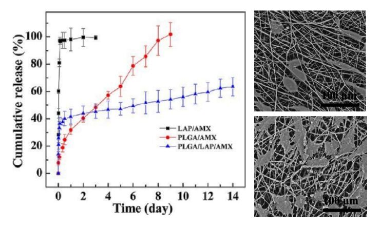
[20] | Wang S, Zheng F, Huang Y, et al. (2012) Encapsulation of amoxicillin within laponite-doped poly(lactic-co-glycolic acid) nanofibers: preparation, characterization, and antibacterial activity. Acs Appl Mater Interfaces 4: 6396-6401. |
[21] |
Özdemir I, Özcan EO, Günal S (2010) Synthesis and Antimicrobial Activity of Novel Ag-N-Heterocyclic Carbene Complexes. Molecules 15: 2499-2508. doi: 10.3390/molecules15042499
![]() |
[22] |
Clement JL, Jarret PS (1994) Antibacterial Silver. Met Based Drugs 1: 467-482. doi: 10.1155/MBD.1994.467
![]() |
[23] |
Tambe SM, Sampath L, Modak SM (2001) In-vitro evaluation of the risk of developing bacterial resistance to antiseptics and antibiotics used in medical devices. J Antimicrob Chemoth 47: 589-598. doi: 10.1093/jac/47.5.589
![]() |
[24] |
Liu JJ, Galettis P, Farr A, et al. (2008) In vitro antitumour and hepatotoxicity profiles of Au(I) and Ag(I) bidentate pyridyl phosphine complexes and relationships to cellular uptake. J Inorg Biochem 102: 303-310. doi: 10.1016/j.jinorgbio.2007.09.003
![]() |
[25] | Jeong L, Kim MH, Jung JY, et al. (2014) Effect of silk fibroin nanofibers containing silver sulfadiazine on wound healing. Int J Nanomed 9: 5277-5287. |
[26] |
Burd A, Kwok CH, Hung SC, et al. (2007) A comparative study of the cyto¬toxicity of silver-based dressings in monolayer cell, tissue explant, and animal model. Wound Repair Regen 15: 94-104. doi: 10.1111/j.1524-475X.2006.00190.x
![]() |
[27] |
Lok CN, Ho CM, Chen R, et al. (2006) Proteomic analysis of the mode of antibacterial action of silver nanoparticles. J Proteome Res 5: 916-924. doi: 10.1021/pr0504079
![]() |
[28] | Lansdown AB (2005) A guide to the properties and uses of silver dressings in wound care. Prof Nurse 20: 41-43. |
[29] |
Vepari C, Kaplan DL (2007) Silk as a biomaterial. Prog Polym Sci 32: 991-1007. doi: 10.1016/j.progpolymsci.2007.05.013
![]() |
[30] |
Kasoju N, Bora U (2012) Silk fibroin in tissue engineering. Adv Healthc Mater 1: 393-412. doi: 10.1002/adhm.201200097
![]() |
[31] |
Dong G, Xiao X, Liu X, et al. (2009) Functional Ag porous films prepared by electrospinning. J Appl Surf Sci 255: 7623-7626. doi: 10.1016/j.apsusc.2009.04.039
![]() |
[32] |
Xu X, Yang Q, Wang Y, el al. (2006) Biodegradable electrospun poly(l-lactide) fibers containing antibacterial silver nanoparticles. Eur Polym J 42: 2081-2087. doi: 10.1016/j.eurpolymj.2006.03.032
![]() |
[33] |
Son WK, Youk JH, Park WH (2006) Antimicrobial cellulose acetate nanofibers containing silver nanoparticles. Carbohyd Polym 65: 430-434. doi: 10.1016/j.carbpol.2006.01.037
![]() |
[34] |
Lala NL, Ramaseshan R, Bojun L, et al. (2007) Fabrication of nanofibers with antimicrobial functionality used as filters: protection against bacterial contaminants. Biotechnol Bioeng 97: 1357-1365. doi: 10.1002/bit.21351
![]() |
[35] | Yang QB, Li DM, Hong YL, el al. (2003) Preparation and characterization of a PAN nanofibre containing Ag nanoparticles via electrospinning Proceedings of the 2002 International Conference on Science and Technology of Synthetic Metals, Elsevier SA, Lausanne, Switzerland, 973-974. |
[36] |
Sheikh FA, Barakat NAM, Kanjwal MA, el al. (2009) Electrospun antimicrobial polyurethane nanofibers containing silver nanoparticles for biotechnological applications. Macromol Res 17: 688-696. doi: 10.1007/BF03218929
![]() |
[37] | Gliscinska E, Gutarowska B, Brycki B, el al. (2012) Electrospun Polyacrylonitrile Nanofibers Modified by Quaternary Ammonium Salts. J Appl Polym Sci 128: 767-775. |
[38] |
Yarin AL, Zussman E (2004) Upward needleless electrospinning of multiple nanofibers. Polymer 45: 2977-2980. doi: 10.1016/j.polymer.2004.02.066
![]() |
[39] |
Nomiya K, Tsuda K, Sudoh T, el al. (1997) Ag(I)-N bond-containing compound showing wide spectra in effective antimicrobial activities: Polymeric silver(I) imidazolate. J Inorg Biochem 68: 39-44. doi: 10.1016/S0162-0134(97)00006-8
![]() |
[40] | Nomiya K, Noguchi R, Oda M (2000) Synthesis and crystal structure of coinage metal(I) complexes with tetrazole (Htetz) and triphenylphosphine ligands, and their antimicrobial activities. A helical polymer of silver(I) complex [Ag(tetz)(PPh3)2]n and a monomeric gold(I) complex [Au(tetz)(PPh3)]. Inorg Chim Acta 298: 24-32. |
[41] |
Atiyeh BS, Ioannovich J, Al-Amm CA, el al. (2002) Management of acute and chronic open wounds: the importance of moist environment in opimal wound healing. Curr Pharm Biotechnol 3: 179-195. doi: 10.2174/1389201023378283
![]() |
[42] |
Akhavan O, Ghaderi E (2009) Enhancement of antibacterial properties of Ag nanorods by electric field. Sci Technol Adv Mat 10: 015003. doi: 10.1088/1468-6996/10/1/015003
![]() |
[43] |
Tijing LD, Amarjargal A, Jiang Z (2013) Antibacterial tourmaline nanoparticles/polyurethane hybrid mat decorated with silver nanoparticles prepared by electrospinning and UV photoreduction. Curr Appl Phys 13: 205-210. doi: 10.1016/j.cap.2012.07.011
![]() |
[44] |
Raffi M, Mehrwan S, Bhatti TM, et al. (2010) Investigations into the antibacterial behavior of copper nanoparticles against Escherichia coli. Ann Microbiol 60: 75-80. doi: 10.1007/s13213-010-0015-6
![]() |
[45] |
Zhong W, Zishena W, Zhenhuana Y, et al. (1994) Synthesis, characterization and antifungal activity of copper (II), zinc (II), cobalt (II) and nickel (II) complexes derived from 2-chlorobenzaldehyde and glycine. Synth React Inorg Met-Org Chem 24: 1453-1460. doi: 10.1080/00945719408002572
![]() |
[46] |
Sheikh FA, Kanjwal MA, Saran S, et al. (2011) Polyurethane nanofibers containing copper nanoparticles as future materials. Appl Surf Sci 257: 3020-3026. doi: 10.1016/j.apsusc.2010.10.110
![]() |
[47] |
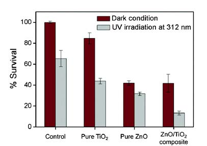
Hwang SH, Song J, Jung Y, et al. (2011) Electrospun ZnO/TiO2 composite nanofibers as a bactericidal agent. J Chem Commun 47: 9164-9166. doi: 10.1039/c1cc12872h
![]() |
[48] |
Lee S (2009) Multifunctionality of layered fabric systems based on electrospun polyurethane/zinc oxide nanocomposite fibers. J Appl Polym Sci 114: 3652-3658. doi: 10.1002/app.30778
![]() |
[49] |
Lee K, Lee S (2012) Multifunctionality of poly(vinyl alcohol) nanofiber webs containing titanium dioxide. J Appl Polym Sci 124: 4038-4046. doi: 10.1002/app.34929
![]() |
[50] | Yu W, Lan CH, Wang SJ, et al. (2010), Influence of Zinc oxide nanoparticles on the crystallization behavior of electrospun poly(3-hydroxybutyrate-co-3-hydroxyvalerate) nanofibers. Polymer 51: 2403. |
[51] |
Drew C, Liu X, Ziegler D, et al. (2003) Metal oxide-coated polymer nanofibers. Nano Lett 3: 143-147. doi: 10.1021/nl025850m
![]() |
[52] |
Horzum N, Mari M, Wagner M, et al. (2015) Controlled surface mineralization of metal oxides on nanofibers. RSC Adv 5: 37340-37345. doi: 10.1039/C5RA02140E
![]() |
[53] |
Klabunde KJ, Stark J, Koper O, et al. (1996) Nanocrystals as stoichiometric reagents with unique surface chemistry. J Phys Chem 100: 12142-12153. doi: 10.1021/jp960224x
![]() |
[54] |
Stoimenov PK, Klinger RL, Marchin GL (2002) Metal Oxide Nanoparticles as Bactericidal Agents. Langmuir 18: 6679-6686. doi: 10.1021/la0202374
![]() |
[55] | Koper O, Klabunde J, Marchin G, et al. (2012) Nanoscale Powders and Formulations with Biocidal Activity Toward Spores and Vegetative Cells of Bacillus Species, Viruses, and Toxins. Curr Microbiol 44: 49-55. |
[56] | McDonnell G, Russell AD (1999) Antiseptics and disinfectants: activity, action, and resistance. Clin Microbiol Rev 12: 147-179. |
[57] | Kügler R, Bouloussa O, Rondelez F (2005) Evidence of a charge-density threshold for optimum Synthesis and antimicrobial activity of modified poly(glycidyl methacrylate-co-2-hydroxy -ethyl methacrylate) derivatives with quaternary ammonium and phosphonium salts. J Polym Sci Pol Chem 40: 2384-2393. |
[58] | Kenawy ER, Abdel-Hay FI, El-Shanshoury A, et al. (2002) Biologically active polymers. V. Synthesis and antimicrobial activity of modified poly(glycidyl methacrylate-co-2-hydroxyethyl methacrylate) derivatives with quaternary ammonium and phosphonium salts. J Polym Sci Part A: Polym Chem 40: 2384-2393. |
[59] |
Kenawy ER, Mahmoud YAG (2003) Biological active polymers. Macromol Biosci 3: 107-116. doi: 10.1002/mabi.200390016
![]() |
[60] |
Lundin JG, Coneski PN, Fulmer PA, et al. (2014) Relationship between surface concentration of amphiphilic quaternary ammonium biocides in electrospun polymer fibers and biocidal activity. React Funct Polym 77: 39-46. doi: 10.1016/j.reactfunctpolym.2014.02.004
![]() |
[61] |
Arumugam GK, Khan S, Heiden PA (2009) Comparison of the Effects of an Ionic Liquid and Other Salts on the Properties of Electrospun Fibers, 2-Poly(vinyl alcohol). Macromol Mater Eng 294: 45-53. doi: 10.1002/mame.200800199
![]() |
[62] |
You Y, Lee SJ, Min BM, et al. (2006) Effect of solution properties on nanofibrous structure of electrospun poly(lactic-co-glycolic acid). J Appl Polym Sci 99: 1214-1221. doi: 10.1002/app.22602
![]() |
[63] |
Tong HW, Wang M (2011) Electrospinning of poly(hydroxybutyrate-co-hydroxyvalerate) fibrous scaffolds for tissue engineering applications: effects of electrospinning parameters and solution properties. J Macromol Sci 50: 1535-1558. doi: 10.1080/00222348.2010.541008
![]() |
[64] |
Park JA, Kim SB (2015) Preparation and characterization of antimicrobial electrospun poly(vinyl alcohol) nanofibers containing benzyl triethylammonium chloride. React Funct Polym 93: 30-37. doi: 10.1016/j.reactfunctpolym.2015.05.008
![]() |
[65] |
Kim SJ, Nam YS, Rhee DM, et al. (2007) Preparation and characterization of antimicrobial polycarbonate nanofibrous membrane. Eur Polym J 43: 3146-3152. doi: 10.1016/j.eurpolymj.2007.04.046
![]() |
[66] |
Nicosia A, Gieparda W, Foksowicz-Flaczyk J, et al. (2015) Air filtration and antimicrobial capabilities of electrospun PLA/PHB containing ionic liquid. Sep Purif Technol 154: 154-160. doi: 10.1016/j.seppur.2015.09.037
![]() |
[67] |
Buruiana EC, Buruiana T (2002) Recent developments in polyurethane cationomers. Photoisomerization reactions in azoaromatic polycations. J Photoch Photobiol A: Chem 151: 237-252. doi: 10.1016/S1010-6030(02)00181-8
![]() |
[68] |
Uykun N, Ergal I, Kurt H, et al. (2014) Electrospun antibacterial nanofibrous polyvinylpyrrolidone/ cetyltrimethylammonium bromide membranes for biomedical applications. J Bioact Compat Pol 29: 382-397. doi: 10.1177/0883911514535153
![]() |
[69] |
Qun XL, Fanf Y, Shan Y, et al. (2010) Antibacterial Nanofibers of Self-quaternized Block Copolymers of 4-Vinyl Pyridine and Pentachlorophenyl Acrylate. High Perform Polym 22: 359-376. doi: 10.1177/0954008309104776
![]() |
[70] |
Cashion MP, Li X, Geng Y, at al. (2010) Gemini Surfactant Electrospun Membranes. Langmuir 26: 678-683. doi: 10.1021/la902287b
![]() |
[71] |
Singh G, Bittner AM, Loscher S, et al. (2008) Electrospinning of diphenylalanine nanotube. Adv Mater 20: 2332-2336. doi: 10.1002/adma.200702802
![]() |
[72] |
Worley SD, Williams DE (1988) Halamine Water Disinfectants. Crit Rev Environ Control 18: 133-175. doi: 10.1080/10643388809388345
![]() |
[73] |
Song J, Jang J (2014) Antimicrobial polymer nanostructures: Synthetic route, mechanism of action and perspective. Adv Colloid Interface Sci 203: 37-50. doi: 10.1016/j.cis.2013.11.007
![]() |
[74] |
Cerkez I, Worley SD, Broughton RM, et al. Huang (2013) Rechargeable antimicrobial coatings for poly(lactic acid) nonwoven fabrics. Polymer 54: 536-541. doi: 10.1016/j.polymer.2012.11.049
![]() |
[75] |
Chen Z, Sun Y (2005) N-Chloro-Hindered Amines as Multifunctional Polymer Additives. Macromolecules 38: 8116-8119. doi: 10.1021/ma050874b
![]() |
[76] | Chen Z, Sun Y (2005) Antimicrobial Functions of N-Chloro-Hindered Amines. Polym Preprint 46: 835-836. |
[77] |
Dong A, Zhang Q, Wang T, et al. (2010) Immobilization of cyclic N-halamine on polystyrene-functionalized silica nanoparticles: synthesis, characterization, and biocidal activity. J Phys Chem C 114: 17298-17303. doi: 10.1021/jp104083h
![]() |
[78] |
Kang J, Han J, Gao Y, et al. (2015) Unexpected Enhancement in Antibacterial Activity of N-Halamine Polymers from Spheres to Fibers. ACS Appl Mater Interfaces 7: 17516-17526. doi: 10.1021/acsami.5b05429
![]() |
[79] |
Sun X, Zhang L, Cao Z, et al. (2010) Electrospun Composite Nanofiber Fabrics Containing Uniformly Dispersed Antimicrobial Agents As an Innovative Type of Polymeric Materials with Superior Antimicrobial Efficacy. ACS Appl Mater Interfaces 2: 952-956. doi: 10.1021/am100018k
![]() |
[80] |
Tan K, Obendorf SK (2007) Fabrication and evaluation of electrospun antimicrobial nylon 6 membranes. J Membrane Sci 305: 287-298. doi: 10.1016/j.memsci.2007.08.015
![]() |
[81] | Dickerson MB, Sierra AA, Bedford NM, et al. (2013) Keratin-based antimicrobial textiles, films, and nanofibers. J Mater Chem B 1: 5505-5514. |
[82] |
Fan X, Jiang Q, Sun Z, et al. (2015) Preparation and Characterization of Electrospun Antimicrobial Fibrous Membranes Based on Polyhydroxybutyrate (PHB). Fiber Polym 16: 1751-1758. doi: 10.1007/s12221-015-5108-1
![]() |
[83] |
Ignatova M, Rashkov I, Manolova N (2013) Drug-loaded electrospun materials in wound-dressing applications and in local cancer treatment. Expert Opin Drug Del 10: 469-483. doi: 10.1517/17425247.2013.758103
![]() |
[84] |
Kim K, Luu YK, Chang C et al. (2004) Incorporation and controlled release of a hydrophilic antibiotic using poly(lactide-co-glycolide)-based electrospun nanofibrous scaffolds. J Control Release 98: 47-56. doi: 10.1016/j.jconrel.2004.04.009
![]() |
[85] |
Yoo HS, Kim TG, Park TG (2009) Surface-functionalized electrospun nanofibers for tissue engineering and drug delivery. Adv Drug Deliver Rev 61: 1033-1042. doi: 10.1016/j.addr.2009.07.007
![]() |
[86] |
Zong XH, Li S, Chen E, at al. (2004) Prevention of postsurgery-induced abdominal adhesions by electrospun bioabsorbable nanofibrous poly(lactide-co-glycolide)-based membranes. Ann Surg 240: 910-915. doi: 10.1097/01.sla.0000143302.48223.7e
![]() |
[87] |
Hong Y, Fujimoto K, Hashizume R, et al. (2008) Generating elastic, biodegradable polyurethane/poly(lactide-co-glycolide) fibrous sheets with controlled antibiotic release via two-stream electrospinning. Biomacromolecules 9: 1200-1207. doi: 10.1021/bm701201w
![]() |
[88] |
Thakur RA, Florek CA, Kohn J, et al. (2008) Electrospun nanofibrous polymeric scaffold with targeted drug release profiles for potential application as wound dressing. Int J Pharm 364: 87-93. doi: 10.1016/j.ijpharm.2008.07.033
![]() |
[89] |
Gilchrist SE, Lange D, Letchford DK, et al. (2013) Fusidic acid and rifampicin co-loaded PLGA nanofibers for the prevention of orthopedic implant associated infections. J Control Release 170: 64-73. doi: 10.1016/j.jconrel.2013.04.012
![]() |
[90] |
Qi R, Guo R, Shen M, et al. (2010) Electrospun poly(lactic-co-glycolic acid)/halloysite nanotube composite nanofibers for drug encapsulation and sustained release. J Mater Chem 20: 10622-10629. doi: 10.1039/c0jm01328e
![]() |
[91] |
Moghe AK, Gupta BS (2008) Co‐axial Electrospinning for Nanofiber Structures: Preparation and Applications. Polym Rev 48: 353-377. doi: 10.1080/15583720802022257
![]() |
[92] |
Viseras C, Cerezo P, Sanchez R, et al. (2010) Current challenges in clay minerals for drug delivery. Appl Clay Sci 48: 291-295. doi: 10.1016/j.clay.2010.01.007
![]() |
[93] |
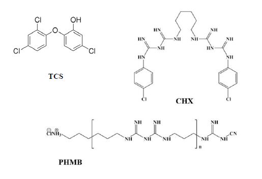
McMurry LM, Oethinger M, Levy SB (1998) Triclosan targets lipid synthesis. Nature 394: 531-532. doi: 10.1038/28970
![]() |
[94] | Green JBD, Fulghum T, Nordhaus MA (2011, Immobilized antimicrobial agents: a critical perspective, In: Science Against Microbial Pathogens: Communicating Current Research and Technological Advances, Formatex Microbiology Books Series, Méndez-Vila E, Ed., Badajoz (Spain). |
[95] |
Kaehn K (2010) Polihexanide: A Safe and Highly Effective Biocide. Skin Pharmacol Physiol 23: 7-16. doi: 10.1159/000318237
![]() |
[96] |
Gilbert P, Pemberton D, Wilkinson DE (1990) Synergism within polyhexamethylene biguanide biocide formulations. J Appl Bacteriol 69: 593-598. doi: 10.1111/j.1365-2672.1990.tb01553.x
![]() |
[97] |
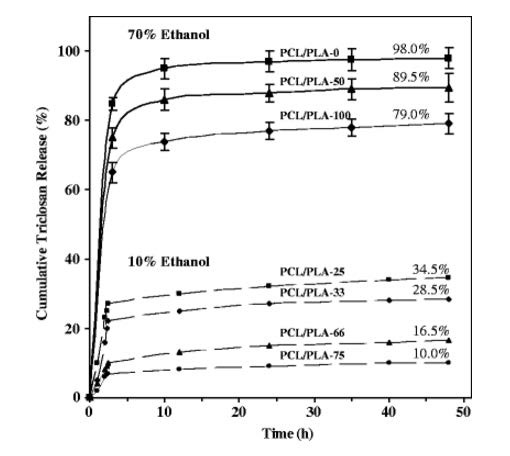
del Valle LJ, Camps R, Díaz A, et al. (2011) Electrospinning of polylactide and polycaprolactone mixtures for preparation of materials with tunable drug release properties. J Polym Res 18: 1903-1917. doi: 10.1007/s10965-011-9597-3
![]() |
[98] |
del Valle LJ, Díaz A, Royo M, et al. (2012) Biodegradable polyesters reinforced with triclosan loaded polylactide micro/nanofibers: Properties, release and biocompatibility. Express Polym Lett 6: 266-282. doi: 10.3144/expresspolymlett.2012.30
![]() |
[99] |
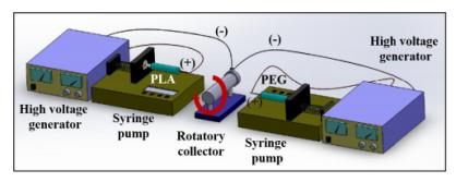
Llorens E, Bellmunt S, del Valle LJ, et al. (2014) Scaffolds constituted by mixed polylactide and poly(ethylene glycol) electrospun microfibers. J Polym Res 21: 603. doi: 10.1007/s10965-014-0603-4
![]() |
[100] |
Llorens E, Ibañez H, del Valle LJ, et al. (2015) Biocompatibility and drug release behavior of scaffolds prepared by coaxial electrospinning of poly(butylene succinate) and polyethylene glycol. Mater Sci Eng C 49: 472-484. doi: 10.1016/j.msec.2015.01.039
![]() |
[101] |
Llorens E, del Valle LJ, Puiggalí J (2015) Electrospun scaffolds of polylactide with a different enantiomeric content and loaded with anti-inflammatory and antibacterial drugs. Macromol Res 23: 636-648. doi: 10.1007/s13233-015-3082-5
![]() |
[102] |
Veiga M, Merino M, Cirri M. et al. (2005) Comparative study on triclosan interactions in solution and in the solid state with natural and chemically modified cyclodextrins. J Incl Phenom Macrocycl Chem 53: 77-83. doi: 10.1007/s10847-005-1047-6
![]() |
[103] |
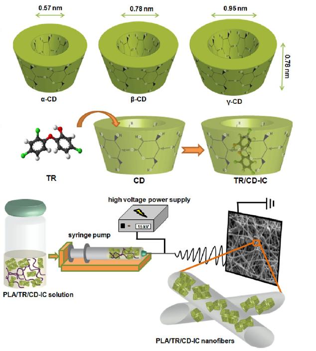
Kayaci F, Umu OCO, Tekinay T, et al. (2013) Antibacterial electrospun Poly(lactic acid) (PLA) nanofibrous webs incorporating triclosan/cyclodextrin inclusion Complexes. J Agric Food Chem 61: 3901-3908. doi: 10.1021/jf400440b
![]() |
[104] |
Celebioglu A, Umu OCO, Tekinay T, et al. (2014) Antibacterial electrospun nanofibers from triclosan/cyclodextrin inclusion complexes. Colloid Surface B 116: 612-619. doi: 10.1016/j.colsurfb.2013.10.029
![]() |
[105] |
Chen L, Bromberg L, Hatton TA (2008) Electrospun cellulose acetate fibers containing chlorhexidine as a bactericide. Polymer 49: 1266-1275. doi: 10.1016/j.polymer.2008.01.003
![]() |
[106] |
Ignatova M, Stoilova O, N Manolova N, et al. (2010) Electrospun mats from styrene/maleic anhydride copolymers: Modification with amines and assessment of antimicrobial activity. Macromol Biosci 10: 944-954. doi: 10.1002/mabi.200900433
![]() |
[107] |
Fernandes JG, Correia DM, Botelho G, et al. (2014) PHB-PEO electrospun fiber membranes containing chlorhexidine for drug delivery applications. Polym Test 34: 64-71. doi: 10.1016/j.polymertesting.2013.12.007
![]() |
[108] | del Valle LJ, Roa M, Díaz A, et al. (2012) Electrospun nanofibers of a degradable poly(ester amide). Scaffolds loaded with antimicrobial agents. J Polym Res 19: 9792. |
[109] |
Díaz A, Katsarava R, Puiggalí J (2014) Synthesis, properties and applications of biodegradable polymers derived from diols and dicarboxylic Acids: From Polyesters to poly(ester amide)s. Int J Mol Sci 15: 7064-7123. doi: 10.3390/ijms15057064
![]() |
[110] | Rodríguez-Galán A, Franco L, Puiggalí J (2011) Degradable poly(ester amide)s for biomedical applications. Polymers 3: 65-99. |
[111] |
Murase SK, del Valle LJ, Kobauri S, et al. (2015) Electrospun fibrous mats from a L-phenylalanine based poly(ester amide): Drug delivery and accelerated degradation by loading enzymes. Polym Degrad Stab 119: 275-287. doi: 10.1016/j.polymdegradstab.2015.05.018
![]() |
[112] |
Díaz A, del Valle LJ, Tugushi D, et al. (2015) New poly(ester urea) derived from L-leucine: Electrospun scaffolds loaded with antibacterial drugs and enzymes. Mater Sci Eng C 46: 450-462. doi: 10.1016/j.msec.2014.10.055
![]() |
[113] | Saha K, Butola BS, Joshi M (2014) Drug-loaded polyurethane/clay nanocomposite nanofibers for topical drug-delivery application. J Appl Polym Sci 131: 40230. |
[114] |
Llorens E, Calderón S, del Valle LJ, et al. (2015) Polybiguanide (PHMB) loaded in PLA scaffolds displaying high hydrophobic, biocompatibility and antibacterial properties. Mater Sci Eng C 50: 74-84. doi: 10.1016/j.msec.2015.01.100
![]() |
[115] | Dash M, Chiellini F, Ottenbrite RM, et al. (2007) Chitosan-a versatile semi-synthetic polymer in biomedical applications. Prog Polym Sci 36: 981-1014. |
[116] | Fischer TH, Bode AP, Demcheva M, et al. (2007) Hemostatic properties of glucosamine-based materials. J Biomed Mater Res A 80: 167-174. |
[117] | Muzzarelli RAA, Belcher R, Freisers H, In: Chitosan in natural chelating polymer; alginic acid, chitin and chitosan, Pergamon Press, Oxford, Pergamon Press, Oxford, 1973, 144-176. |
[118] |
Geng X, Kwon OH, Jang J (2005) Electrospinning of chitosan dissolved in concentrated acetic acid solution. Biomaterials 26: 5427-5432. doi: 10.1016/j.biomaterials.2005.01.066
![]() |
[119] | Spasova M, Manolova N, Paneva D, et al (2004) Preparation of chitosan-containing nanofibres by electrospinning of chitosan/poly(ethylene oxide) blend solutions. e-Polymers 4: 624-635. |
[120] |
Bhattaraia B, Edmondson D, Veiseh O, et al. (2005) Electrospun chitosan-based nanofibers and their cellular compatibility. Biomaterials 26: 6176-6184. doi: 10.1016/j.biomaterials.2005.03.027
![]() |
[121] |
Ignatova M, Starbova K, Markova N, et al. (2006) Electrospun nano-fibre mats with antibacterial properties from quaternised chitosan and poly(vinyl alcohol). Carbohyd Res 341: 2098-2107. doi: 10.1016/j.carres.2006.05.006
![]() |
[122] |
Min BM, Lee SW, Lim JN, et al. (2004) Chitin and chitosan nanofibers: Electrospinning of chitin and deacetylation of chitin nanofibers. Polymer 45: 7137-7142. doi: 10.1016/j.polymer.2004.08.048
![]() |
[123] |
Ohkawa K, Cha D, Kim H, et al. (2004) Electrospinning of chitosan. Macromol Rapid Comm 25: 1600-1605. doi: 10.1002/marc.200400253
![]() |
[124] |
Neamnark A, Rujiravaniti R, Supaphol P (2006) Electrospinning of hexanoyl chitosan. Carbohydrate. Polymers 66: 298-305. doi: 10.1016/j.carbpol.2006.03.015
![]() |
[125] |
Homayoni H, Ravandi SH, Valizadeh M (2009) Electrospinning of chitosan nanofibers: Processing optimization. Carbohyd Polym 77: 656-661. doi: 10.1016/j.carbpol.2009.02.008
![]() |
[126] |
Zong X, Kim K, Fang D, et al. (2002) Structure and process relationship on electrospun bioabsorbable nanofiber membranes. Polymer 43: 4403-4412. doi: 10.1016/S0032-3861(02)00275-6
![]() |
[127] |
Au HT, Pham LN, Vu THT, et al. (2012) Fabrication of an antibacterial non-woven mat of a poly(lactic acid)/chitosan blend by electrospinning. Macromol Res 20: 51-58. doi: 10.1007/s13233-012-0010-9
![]() |
[128] |
Shalumon KT, Anulekha KH, Girish CM, et al. (2010) Single step electrospinning of chitosan/poly(caprolactone) nanofibers using formic acid/acetone solvent mixture. Carbohyd Polym 80: 413-417. doi: 10.1016/j.carbpol.2009.11.039
![]() |
[129] |
Cooper A, Oldinski R, Ma H, et al. (2013) Chitosan-based nanofibrous membranes for antibacterial filter applications. Carbohyd Polym 92: 254-259. doi: 10.1016/j.carbpol.2012.08.114
![]() |
[130] |
Zheng H, Du Y, Yu J, et al. (2001) Preparation and characterization of chitosan/poly(vinyl alcohol) blend fibers. J Appl Polym Sci 80: 2558-2565. doi: 10.1002/app.1365
![]() |
[131] |
Chuang WY, Young TH, Yao CH, et al. (1999) Properties of the poly(vinyl alcohol)/chitosan blend and its effect on the culture of fibroblast in vitro. Biomaterials 20: 1479-1487. doi: 10.1016/S0142-9612(99)00054-X
![]() |
[132] |
Jia YT, Gong J, Gu XH, et al. (2007) Fabrication and characterization of poly(vinyl alcohol)/chitosan blend nanofibers produced by electrospinning method. Carbohyd Polym 67: 403-409. doi: 10.1016/j.carbpol.2006.06.010
![]() |
[133] |
Zhang H, Li S, White CJB, et al. (2009) Studies on electrospun nylon-6/chitosan complex nanofiber interactions. Electrochim Acta 54: 5739-5745. doi: 10.1016/j.electacta.2009.05.021
![]() |
[134] |
Lin SJ, Hsiao WU, Jee SH, et al. (2006) Study on the effects of nylon–chitosan-blended membranes on the spheroid-forming activity of human melanocytes. Biomaterials 27: 5079-5088. doi: 10.1016/j.biomaterials.2006.05.035
![]() |
[135] |
Ma Z, Kotaki M, Yong T, et al. (2005) Surface engineering of electrospun polyethylene terephthalate (PET) nanofibers towards development of a new material for blood vessel engineering. Biomaterials 26: 2527-2536. doi: 10.1016/j.biomaterials.2004.07.026
![]() |
[136] |
Jung KH, Huh MW, Meng W, et al. (2007) Preparation and antibacterial activity of PET/chitosan nanofibrous mats using an electrospinning technique. J Appl Polym Sci 105: 2816-2823. doi: 10.1002/app.25594
![]() |
[137] |
An J, Zhang H, Zhang JT, et al. (2009) Preparation and antibacterial activity of electrospun chitosan/poly(ethylene oxide) membranes containing silver nanoparticles. Colloid Polym Sci 287: 1425-1434. doi: 10.1007/s00396-009-2108-y
![]() |
[138] |
Zhuang XP, Cheng BW, Kang WM, et al. (2010) Electrospun chitosan/gelatin nanofibers containing silver nanoparticles. Carbohyd Polym 82: 524-527. doi: 10.1016/j.carbpol.2010.04.085
![]() |
[139] |
Cai ZX, Mo XM, Zhang KH, et al. (2010) Fabrication of chitosan/silk fibroin composite nanofibers for wound dressing applications. Int J Mol Sci 11: 3529-3539. doi: 10.3390/ijms11093529
![]() |
[140] |
Alipour SM, Nouri M, Mokhtari J, et al. (2009) Electrospinning of poly(vinyl alcohol)–water-soluble quaternized chitosan derivative blend. Carbohyd Res 344: 2496-2501. doi: 10.1016/j.carres.2009.10.004
![]() |
[141] |
Fu GD, Yao F, Li Z, et al. (2008) Solvent-resistant antibacterial microfibers of self-quaternized block copolymers from atom transfer radical polymerization and electrospinning. J Mater Chem 18: 859-867. doi: 10.1039/b716127a
![]() |
[142] |
Parfitt T (2005) Georgia: an unlikely stronghold for bacteriophage therapy. The Lancet 365: 2166-2167. doi: 10.1016/S0140-6736(05)66759-1
![]() |
[143] | Sulakvelidze A, Kutter E (2005) Bacteriophage therapy in humans, In: Bacteriophages: Biology and Applications, Kutter E, Sulakvelidze A, Eds., CRC Press, Boca Raton, FL, 381-436. |
[144] |
Kutter E, De Vos D, Gvasalia G, et al. (2010) Phage therapy in clinical practice: treatment of human infections. Curr Pharm Biotechnol 11: 69-86. doi: 10.2174/138920110790725401
![]() |
[145] |
Abedon S, Kuhl S, Blasdel B, et al. (2011) Phage treatment of human infections. Bacteriophage 1: 66-85. doi: 10.4161/bact.1.2.15845
![]() |
[146] | FDA (2006) FDA approval of Listeria-specific bacteriophage preparation on ready-to-eat (RTE) meat and poultry products. FDA, Washington, DC. |
[147] |
Frykberg RG, Armstrong DG, Giurini J, et al. (2000) Diabetic foot disorders: a clinical practice guideline. J Foot Ankle Surg 39: S1-S60. doi: 10.1016/S1067-2516(00)80057-5
![]() |
[148] |
Anany H, Chen W, Pelton R (2011) Biocontrol of Listeria monocytogenes and Escherichia coli O157:H7 in Meat by Using Phages Immobilized on Modified Cellulose Membranes. Appl Environ Microb 77: 6379-6387. doi: 10.1128/AEM.05493-11
![]() |
[149] |
Markoishvili K, Tsitlanadze G, Katsarava R, et al. (2002) A novel sustained-release matrix based on biodegradable poly(ester amide)s and impregnated with bacteriophages and an antibiotic shows promise in management of infected venous stasis ulcers and other poorly healing wounds. Int J Dermatol 41: 453-458. doi: 10.1046/j.1365-4362.2002.01451.x
![]() |
[150] | Katsarava R, Alavidze Z (2004) Polymer Blends as Biodegradable Matrices for Preparing Biocomposites, US Patent 6,703,040 (Assigned to Intralytix, Inc.). |
[151] | Katsarava R, Gomurashvili Z (2011) Biodegradable Polymers Composed of Naturally Occurring α-Amino Acids, In: Handbook of Biodegradable Polymers—Isolation, Synthesis, Characterization and Applications. Lendlein A, Sisson A, Eds., Wiley-VCH, Verlag GmbH & Co KGaA, Ch. 5. |
[152] |
Jikia D, Chkhaidze N, Imedashvili E, et al. (2005) The use of a novel biodegradable preparation capable of the sustained release of bacteriophages and ciprofloxacin, in the complex treatment of multidrug - resistant Staphylococcus aureus-infected local radiation injuries caused by exposure to Sr90. Clin Exp Dermatol 30: 23-26. doi: 10.1111/j.1365-2230.2004.01600.x
![]() |
[153] |
Puapermpoonsiri U, Spencer J, van der Walle CF (2009) A freeze-dried formulation of bacteriophage encapsulated in biodegradable microspheres. Eur J Pharm Biopharm 72: 26-33. doi: 10.1016/j.ejpb.2008.12.001
![]() |
[154] |
Gervais L, Gel M, Allain B, et al. (2007) Immobilization of biotinylated bacteriophages on biosensor surfaces. Sensor Actuat B-Chem 125: 615-621. doi: 10.1016/j.snb.2007.03.007
![]() |
[155] |
Nanduri V, Balasubramanian S, Sista S, et al. (2007) Highly sensitive phage-based biosensor for the detection of β-galactosidase. Anal Chim Acta 589: 166-172. doi: 10.1016/j.aca.2007.02.071
![]() |
[156] | Tawil N, Sacher E, Rioux D, et al. (2015) Surface Chemistry of Bacteriophage and Laser Ablated Nanoparticle Complexes for Pathogen Detection. J Phys Chem C 119: 14375-14382. |
[157] | Sun W, Brovko L, Griffiths M (2001) Food-borne pathogens. Use of bioluminescent salmonella for assessing the efficiency of Constructed phage-based biosorbent. J Ind Microbiol Biot 27: 126-128. |
[158] |
Cademartiri R, Anany H, Gross I, et al. (2010). Immobilization of bacteriophages on modified silica particles. Biomaterials 31: 1904-1910. doi: 10.1016/j.biomaterials.2009.11.029
![]() |
[159] |
Bennett AR, Davids FGC, Vlahodimou S, et al. (1997) The use of bacteriophage-based systems for the separation and concentration of Salmonella. J Appl Microbiol 83: 259-265. doi: 10.1046/j.1365-2672.1997.00257.x
![]() |
[160] |
Pearson HA, Sahukhal GS, Elasri MO, et al. (2013) Phage-Bacterium War on Polymeric Surfaces: Can Surface-Anchored Bacteriophages Eliminate Microbial Infections? Biomacromolecules 14: 1257-1261. doi: 10.1021/bm400290u
![]() |
[161] |
Dai M, Senecal A, Nugen SR (2014) Electrospun water-soluble polymer nanofibers for the dehydration and storage of sensitive reagents. Nanotechnology 25: 225101. doi: 10.1088/0957-4484/25/22/225101
![]() |
[162] | Korehei R, Kadla J (2011) Incorporating pre-encapsulated bacteriophage in electrospun fibres, 16th International Symposium on Wood, Fiber and Pulping Chemistry, Tianjin, People’s Republic of China. Proceedings ISWFPC 2: 1302-1306. |
[163] |
Lee SW, Belcher AM (2004) Virus-based fabrication of micro- and nanofibers using electrospinning. J Nano Lett 4: 387-390. doi: 10.1021/nl034911t
![]() |
[164] |
Salalha W, Kuhn J, Dror Y, et al. (2006) Encapsulation of bacteria and viruses in electrospun nanofibers. Nanotechnology 17: 4675-4681. doi: 10.1088/0957-4484/17/18/025
![]() |
[165] |
Korehei R, Kadla J (2013) Incorporation of T4 bacteriophage in electrospun fibres. J Appl Microbiol 114: 1425-1434. doi: 10.1111/jam.12158
![]() |
1. | Yang Cao, Hongte Wu, Preparation and performance analysis of polycarboxylate superplasticizer modified with fluorine-containing monomer and silicon dioxide nanoparticles, 2024, 14, 2158-5849, 605, 10.1166/mex.2024.2665 |