Fibonacci signals with timing jitter

D. S. Citrin; D. S. Citrin

doi:10.3934/mine.2023076

Mathematics in Engineering

2023, Volume 5, Issue 4: 1-13. doi: 10.3934/mine.2023076

Previous Article Next Article

Research article

Fibonacci signals with timing jitter

D. S. Citrin ^{1,2
,
,}

1.
School of Electrical and Computer Engineering, Georgia Institute of Technology, Atlanta, Georgia 30332-0250, USA
2.
Georgia Tech-CNRS IRL 2958, Georgia Tech Europe, 2 Rue Marconi, 57070 Metz, France

Received: 18 November 2022 Revised: 05 February 2023 Accepted: 05 February 2023 Published: 17 February 2023

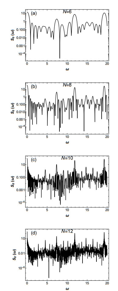
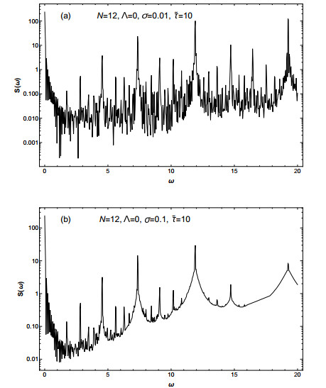
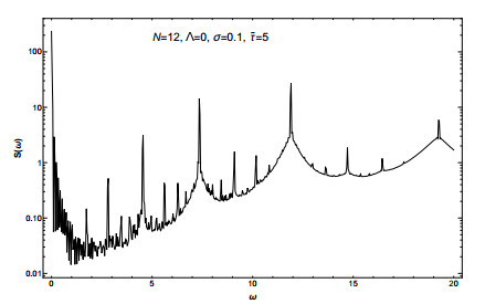
The power spectral density of a signal comprised of a sequence of Dirac $ \delta $-functions at successive times determined by a Fibonacci sequence is the temporal analog of the well known structure factor for a Fibonacci chain. Such a signal is quasi-periodic and, under suitable choice of parameters, is the temporal analog of a one-dimensional quasicrystal. While the effects of disorder in the spatial case of Fibonacci chains has been studied numerically, having an analytically tractable stochastic model is needed both for the spatial and temporal cases to be able to study these effects as model parameters are varied. Here, we consider the effects of errors in where the $ \delta $-functions defining the signal in the temporal case occur, i.e., timing jitter. In this work, we present an analytically tractable theory of how timing jitter affects the power spectral density of Fibonacci signals.
- Fibonacci sequences,
- nonperiodic sampling,
- timing jitter
Citation: D. S. Citrin. Fibonacci signals with timing jitter[J]. Mathematics in Engineering, 2023, 5(4): 1-13. doi: 10.3934/mine.2023076

Related Papers:

Abstract

The power spectral density of a signal comprised of a sequence of Dirac $ \delta $-functions at successive times determined by a Fibonacci sequence is the temporal analog of the well known structure factor for a Fibonacci chain. Such a signal is quasi-periodic and, under suitable choice of parameters, is the temporal analog of a one-dimensional quasicrystal. While the effects of disorder in the spatial case of Fibonacci chains has been studied numerically, having an analytically tractable stochastic model is needed both for the spatial and temporal cases to be able to study these effects as model parameters are varied. Here, we consider the effects of errors in where the $ \delta $-functions defining the signal in the temporal case occur, i.e., timing jitter. In this work, we present an analytically tractable theory of how timing jitter affects the power spectral density of Fibonacci signals.

References

[1]	M. Kohmoto, L. P. Kadanoff, C. Tang, Localization problem in one dimension: mapping and escape, Phys. Rev. Lett., 50 (1983), 1870–1872. https://doi.org/10.1103/PhysRevLett.50.1870 doi: 10.1103/PhysRevLett.50.1870
[2]	S. Ostlund, R. Pandit, D. Rand, H. J. Schellnhuber, E. D. Siggia, One-dimensional Schrödinger equation with an almost periodic potential, Phys. Rev. Lett., 50 (1983), 1873–1876. https://doi.org/10.1103/PhysRevLett.50.1873 doi: 10.1103/PhysRevLett.50.1873
[3]	R. Merlin, K. Bajema, R. Clarke, F.-Y. Juang, P. K. Bhattacharya, Quasiperiodic GaAs-A1As heterostructures, Phys. Rev. Lett., 55 (1985), 1768–1770. https://doi.org/10.1103/PhysRevLett.55.1768 doi: 10.1103/PhysRevLett.55.1768
[4]	J. Todd, R. Merlin, R. Clarke, K. M. Mohanty, J. D. Axe, Synchrotron X-ray study of a Fibonacci superlattice, Phys. Rev. Lett., 57 (1986), 1157–1160. https://doi.org/10.1103/PhysRevLett.57.1157 doi: 10.1103/PhysRevLett.57.1157
[5]	M. C. Valsakumar, V. Kumar, Diffraction from a quasi-crystalline chain, Pramana, 26 (1986), 215–221. https://doi.org/10.1007/BF02845262 doi: 10.1007/BF02845262
[6]	D. Paquet, M. C. Joncour, B. Jusserand, F. Laruelle, F. Mollot, B. Etienne, Structural and optical properties of periodic Fibonacci superlattices, In: Spectroscopy of semiconductor microstructures, Boston: Springer, 1989,223–234. https://doi.org/10.1007/978-1-4757-6565-6_14
[7]	F. Nori, J. P. Rodriguez, Acoustic and electronic properties of one-dimensional quasicrystals, Phys. Rev. B, 34 (1986), 2207–2211. https://doi.org/10.1103/PhysRevB.34.2207 doi: 10.1103/PhysRevB.34.2207
[8]	J. Kollar, A. Sütō, The Kronig-Penney model on a Fibonacci lattice, Phys. Lett. A, 117 (1986), 203–209. https://doi.org/10.1016/0375-9601(86)90741-3 doi: 10.1016/0375-9601(86)90741-3
[9]	V. Kumar, G. Ananthakrishna, Electronic structure of a quasiperiodic superlattice, Phys. Rev. Lett., 59 (1987), 1476–1479. https://doi.org/10.1103/PhysRevLett.59.1476 doi: 10.1103/PhysRevLett.59.1476
[10]	J. P. Lu, J. L. Birman, Electronic structure of a quasiperiodic system, Phys. Rev. B, 36 (1987), 4471–4474. https://doi.org/10.1103/PhysRevB.36.4471 doi: 10.1103/PhysRevB.36.4471
[11]	Q. Niu, F. Nori, Renormalization-group study of one-dimensional quasiperiodic systems, Phys. Rev. Lett., 57 (1986), 2057–2060. https://doi.org/10.1103/PhysRevLett.57.2057 doi: 10.1103/PhysRevLett.57.2057
[12]	L. Chen, G. Hu, R. Tao, Dynamical study of a one-dimensional quasi-crystal, Phys. Lett. A, 117 (1986), 120–122. https://doi.org/10.1016/0375-9601(86)90016-2 doi: 10.1016/0375-9601(86)90016-2
[13]	M. W. C. Dharma-wardana, A. H. MacDonald, D. J. Lockwood, J.-M. Baribeau, D. C. Houghton, Raman scattering in Fibonacci superlattices, Phys. Rev. Lett., 58 (1987), 1761–1764. https://doi.org/10.1103/PhysRevLett.58.1761 doi: 10.1103/PhysRevLett.58.1761
[14]	M. Nakayama, H. Kato, S. Nakashima, Folded acoustic phonons in (AI, Ga)As quasiperiodic superlattices, Phys. Rev. B, 36 (1987), 3472–3474. https://doi.org/10.1103/PhysRevB.36.3472 doi: 10.1103/PhysRevB.36.3472
[15]	K. Bajema, R. Merlin, Raman scattering by acoustic phonons in Fibonacci GaAs-A1As superlattices, Phys. Rev. B, 36 (1987), 4555–4557. https://doi.org/10.1103/PhysRevB.36.4555 doi: 10.1103/PhysRevB.36.4555
[16]	H. Hiramoto, S. Abe, Anomalous quantum diffusion in quasiperiodic potentials, Jpn. J. Appl. Phys., 26 (1987), 665–666. https://doi.org/10.7567/JJAPS.26S3.665 doi: 10.7567/JJAPS.26S3.665
[17]	S. Das Sarma, A. Kobayashi, R. E. Prange, Plasmons in aperiodic structures, Phys. Rev. B, 34 (1986), 5309–5314. https://doi.org/10.1103/PhysRevB.34.5309 doi: 10.1103/PhysRevB.34.5309
[18]	P. Hawrylak, J. J. Quinn, Critical plasmons of a quasiperodic semiconductor superlattice, Phys. Rev. Lett., 57 (1986), 380–383. https://doi.org/10.1103/PhysRevLett.57.380 doi: 10.1103/PhysRevLett.57.380
[19]	M. Goda, Response function and conductance of a Fibonacci lattice, J. Phys. Soc. Jpn., 56 (1987), 1924–1927. https://doi.org/10.1143/JPSJ.56.1924 doi: 10.1143/JPSJ.56.1924
[20]	J. B. Sokoloff, Anomalous electrical conduction in quasicrystals and Fibonacci lattices, Phys. Rev. Lett., 58 (1987), 2267–2270. https://doi.org/10.1103/PhysRevLett.58.2267 doi: 10.1103/PhysRevLett.58.2267
[21]	T. Schneider, A. Politi, D. Wiirtz, Resistance and eigenstates in a tight-binding model with quasiperiodic potential, Z. Phys. B, 66 (1987), 469–473. https://doi.org/10.1007/BF01303896 doi: 10.1007/BF01303896
[22]	D. Lusk, I. Abdulhalim, F. Placido, Omnidirectional reflection from Fibonacci quasi-periodic one-dimensional photonic crystal, Opt. Commun., 198 (2001), 273–279. https://doi.org/10.1016/S0030-4018(01)01531-0 doi: 10.1016/S0030-4018(01)01531-0
[23]	L. Dal Negro, C. J. Oton, Z. Gaburro, L. Pavesi, P. Johnson, A. Lagendijk, et al., Light transport through the band-edge states of Fibonacci quasicrystals, Phys. Rev. Lett., 90 (2003), 055501. https://doi.org/10.1103/PhysRevLett.90.055501 doi: 10.1103/PhysRevLett.90.055501
[24]	D. Levine, P. J. Steinhardt, Quasicrystals: a new class of ordered structures, Phys. Rev. Lett., 53 (1984), 2477–2480. https://doi.org/10.1103/PhysRevLett.53.2477 doi: 10.1103/PhysRevLett.53.2477
[25]	R. Merlin, Raman studies of Fibonacci, thue-morse, and random superlattices, In: Light scattering in solids V, Berlin: Springer, 1989,214–232. https://doi.org/10.1007/BFb0051990
[26]	R. Merlin, Structural and electronic properties of nonperiodic superlattices, IEEE J. Quantum Elect., 24 (1988), 1791–1798. https://doi.org/10.1109/3.7108 doi: 10.1109/3.7108
[27]	A. Jagannathan, The Fibonacci quasicrystal: case study of hidden dimensions and multifracticality, Rev. Mod. Phys., 93 (2021), 045001. https://doi.org/10.1103/RevModPhys.93.045001 doi: 10.1103/RevModPhys.93.045001
[28]	R. K. P. Zia, W. J. Dallas, A simple derivation of quasi-crystalline spectra, J. Phys. A: Math. Gen., 18 (1985), L341–L345. https://doi.org/10.1088/0305-4470/18/7/002 doi: 10.1088/0305-4470/18/7/002
[29]	Y. Liu, R. Riklund, Electronic properties of perfect and non-perfect one-dimensional quasicrystals, Phys. Rev. B, 35 (1987), 6034–6042. https://doi.org/10.1103/PhysRevB.35.6034 doi: 10.1103/PhysRevB.35.6034
[30]	V. Holý, J. Kuběna, K. Ploog, X-ray analysis of structural defects in a semiconductor superlattice, Phys. Status Solidi. B, 162 (1990), 347–361. https://doi.org/10.1002/pssb.2221620204 doi: 10.1002/pssb.2221620204
[31]	M. Lax, Classical noise. V. Noise in self-sustained oscillators, Phys. Rev., 160 (1960), 290–307. https://doi.org/10.1103/PhysRev.160.290 doi: 10.1103/PhysRev.160.290
[32]	R. Adler, A study of locking phenomena in oscillators, Proceedings of the IRE, 43 (1946), 351–357. https://doi.org/10.1109/JRPROC.1946.229930 doi: 10.1109/JRPROC.1946.229930
[33]	H. A. Haus, H. L. Dyckman, Timing of laser pulses produced by combined passive and active mode-locking, Int. J. Electron., 44 (1978), 333–335. https://doi.org/10.1080/00207217808900814 doi: 10.1080/00207217808900814
[34]	A. F. Talla, R. Martinenghi, G. R. Goune Chengui, J. H. Talla Mbé, K. Saleh, A. Coillet, et al., Analysis of phase-locking in narrow-band optoelectronic oscillators with intermediate frequency, IEEE J. Quantum Elect., 51 (2015), 5000108. https://doi.org/10.1109/JQE.2015.2425957 doi: 10.1109/JQE.2015.2425957
[35]	S. N. Karmakar, A. Chakrabarti, R. K. Moitra, Dynamic structure factor of a Fibonacci lattice: a renormalization-group approach, Phys. Rev. B, 46 (1992), 3660–3663. https://doi.org/10.1103/PhysRevB.46.3660 doi: 10.1103/PhysRevB.46.3660
[36]	N. Wiener, Generalized harmonic analysis, Acta Math., 55 (1930), 117–258. https://doi.org/10.1007/BF02546511 doi: 10.1007/BF02546511
[37]	A. Khintchine, Korrelationstheorie der stationären stochastischen Prozesse, Math. Ann., 109 (1934), 604–615. https://doi.org/10.1007/BF01449156 doi: 10.1007/BF01449156
[38]	D. S. Citrin, Connection between optical frequency combs and microwave frequency combs produced by active-mode-locked lasers subject to timing jitter, Phys. Rev. Appl., 16 (2021), 014004. https://doi.org/10.1103/PhysRevApplied.16.014004 doi: 10.1103/PhysRevApplied.16.014004
[39]	A. Guinier, X-ray diffraction in crystals, imperfect crystals, and amorphous bodies, San Francisco: W. H. Freeman, 1963.

Reader Comments

Your name:*

Email:*
© 2023 the Author(s), licensee AIMS Press. This is an open access article distributed under the terms of the Creative Commons Attribution License (http://creativecommons.org/licenses/by/4.0)