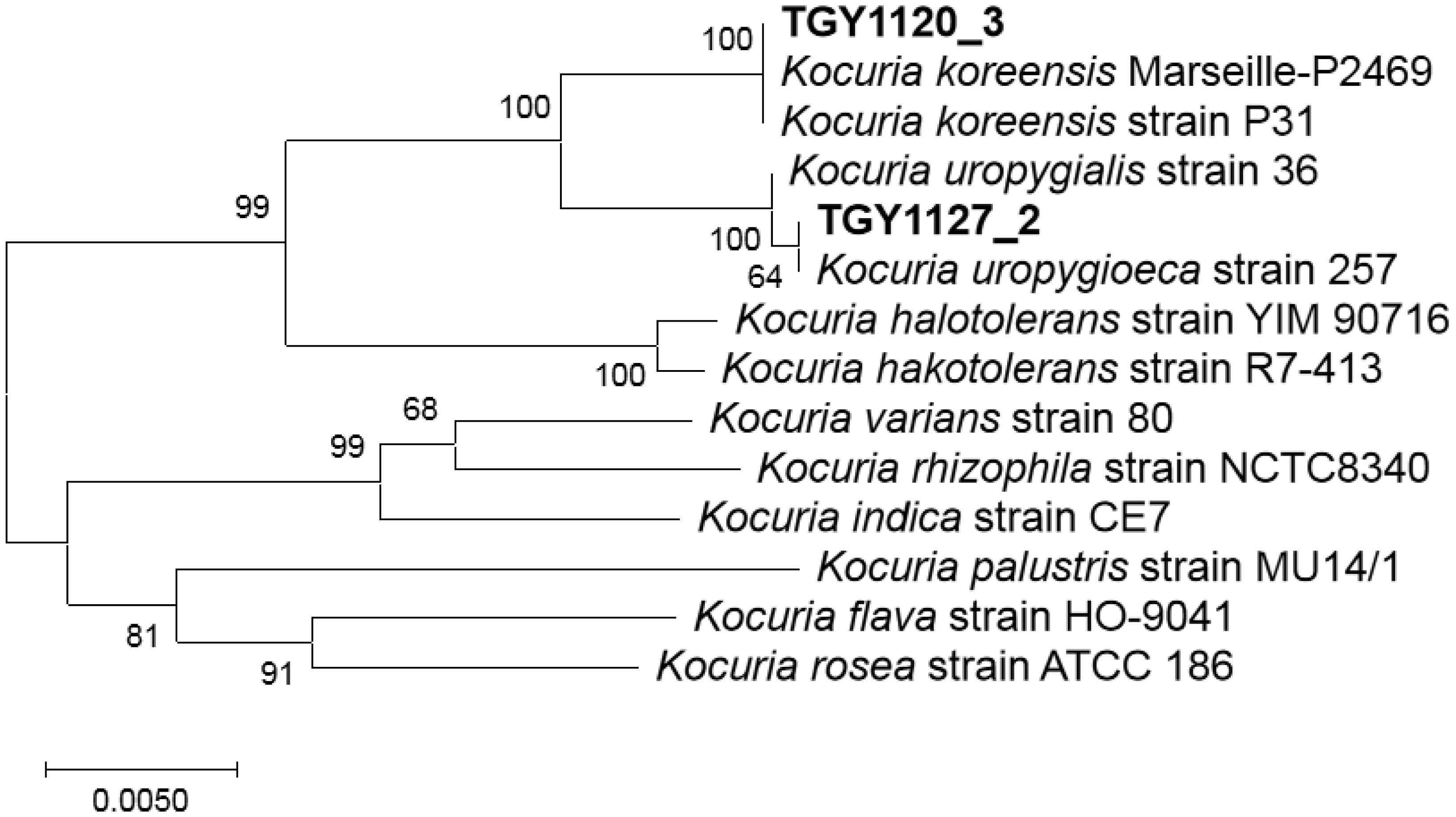
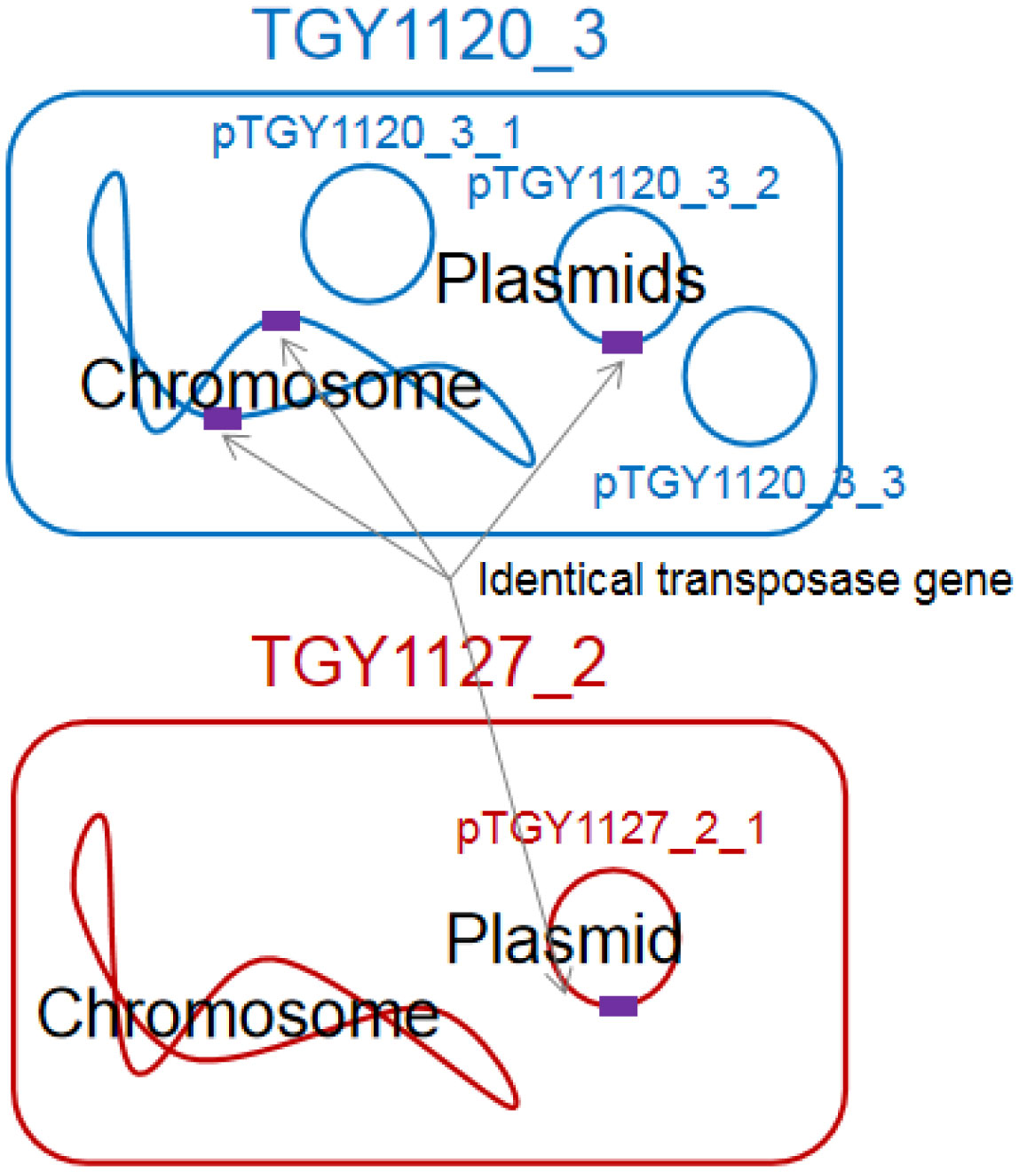
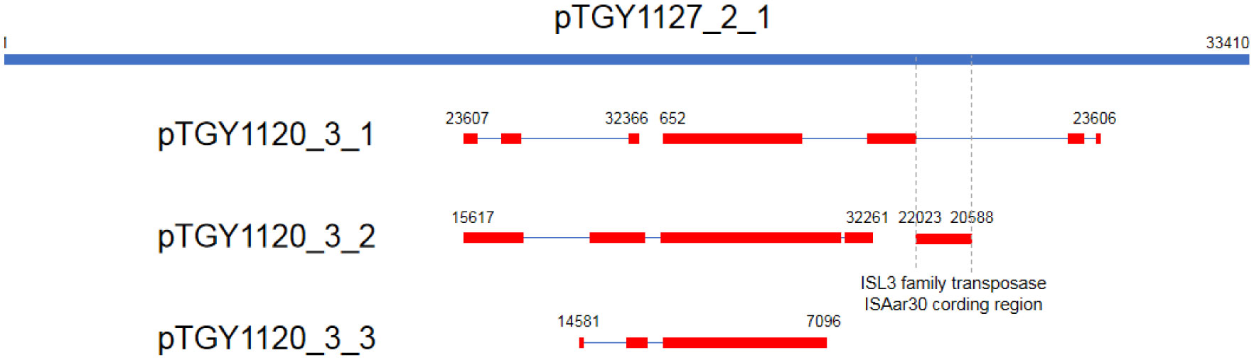
Bacteria belonging to the genus Kocuria were identified as bacteria peculiar to a sake brewery in Toyama, Japan. Comparison of the 16S rRNA gene sequences revealed two groups of Kocuria isolates. Among known species, one group was similar to K. koreensis (Kk type), and the other, K. uropygioeca (Ku type). We determined complete genomic DNA sequences from two isolates, TGY1120_3 and TGY1127_2, which belong to types Kk and Ku, respectively. Comparison of these genomic information showed that these isolates differ at the species level with different genomic characters. Isolate TGY1120_3 comprised one chromosome and three plasmids, and the same transposon coding region was located on two loci on the chromosome and one locus on one plasmid, suggesting that the genetic element may be transferred between the chromosome and plasmid. Isolate TGY1127_2 comprised one chromosome and one plasmid. This plasmid encoded an identical transposase coding region, strongly suggesting that the genetic element may be transferred between these different isolates through plasmids. These four plasmids carried a highly similar region, indicating that they share a common ancestor. Thus, these two isolates may form a community and exchange their genetic information during sake brewing.
Citation: Momoka Terasaki, Yukiko Kimura, Masato Yamada, Hiromi Nishida. Genomic information of Kocuria isolates from sake brewing process[J]. AIMS Microbiology, 2021, 7(1): 114-123. doi: 10.3934/microbiol.2021008
Bacteria belonging to the genus Kocuria were identified as bacteria peculiar to a sake brewery in Toyama, Japan. Comparison of the 16S rRNA gene sequences revealed two groups of Kocuria isolates. Among known species, one group was similar to K. koreensis (Kk type), and the other, K. uropygioeca (Ku type). We determined complete genomic DNA sequences from two isolates, TGY1120_3 and TGY1127_2, which belong to types Kk and Ku, respectively. Comparison of these genomic information showed that these isolates differ at the species level with different genomic characters. Isolate TGY1120_3 comprised one chromosome and three plasmids, and the same transposon coding region was located on two loci on the chromosome and one locus on one plasmid, suggesting that the genetic element may be transferred between the chromosome and plasmid. Isolate TGY1127_2 comprised one chromosome and one plasmid. This plasmid encoded an identical transposase coding region, strongly suggesting that the genetic element may be transferred between these different isolates through plasmids. These four plasmids carried a highly similar region, indicating that they share a common ancestor. Thus, these two isolates may form a community and exchange their genetic information during sake brewing.

| [1] |
Kitagaki H, Kitamoto K (2013) Breeding research on sake yeasts in Japan: history, recent technological advances, and future perspectives. Ann Rev Food Sci Technol 4: 215-235. doi: 10.1146/annurev-food-030212-182545

|
| [2] |
Akao T, Yashiro I, Hosoyama A, et al. (2011) Whole-genome sequencing of sake yeast Saccharomyces cerevisiae Kyokai no. 7. DNA Res 18: 423-434. doi: 10.1093/dnares/dsr029
|
| [3] |
Ohya Y, Kashima M (2019) History, lineage and phenotypic differentiation of sake yeast. Biosci Biotechnol Biochem 83: 1442-1448. doi: 10.1080/09168451.2018.1564620
|
| [4] |
Azumi M, Goto-Yamamoto N (2001) AFLP analysis of type strains and laboratory and industrial strains of Saccharomyces cerevisiae stricto and its application to phenetic clustering. Yeast 18: 1145-1154. doi: 10.1002/yea.767
|
| [5] |
Terasaki M, Fukuyama A, Takahashi Y, et al. (2017) Bacterial DNA detected in Japanese rice wines and the fermentation starters. Curr Microbiol 74: 1432-1437. doi: 10.1007/s00284-017-1337-4
|
| [6] |
Akaike M, Miyagawa H, Kimura Y, et al. (2020) Chemical and bacterial components in sake and sake production process. Curr Microbiol 77: 632-637. doi: 10.1007/s00284-019-01718-4
|
| [7] |
Suzuki K, Asano S, Iijima K, et al. (2008) Sake and beer spoilage lactic acid bacteria—a review. J Inst Brew 114: 209-223. doi: 10.1002/j.2050-0416.2008.tb00331.x
|
| [8] |
Bokulich NA, Ohta M, Lee M, et al. (2014) Indigenous bacteria and fungi drive traditional kimoto sake fermentations. Appl Environ Microbiol 80: 5522-5529. doi: 10.1128/AEM.00663-14
|
| [9] |
Koyanagi T, Nakagawa A, Kiyohara M, et al. (2016) Tracing microbiota changes in yamahai-moto, the traditional Japanese sake starter. Biosci Biotech Biochem 80: 399-406. doi: 10.1080/09168451.2015.1095067
|
| [10] |
Tsuji A, Kozawa M, Tokuda K, et al. (2018) Robust domination of Lactobacillus sakei in microbiota during traditional Japanese sake starter yamahai-moto fermentation and the accompanying changes in metabolites. Curr Microbiol 75: 1498-1505. doi: 10.1007/s00284-018-1551-8
|
| [11] |
Terasaki M, Miyagawa S, Yamada M, et al. (2018) Detection of bacterial DNA during the process of sake production using sokujo-moto. Curr Microbiol 75: 874-879. doi: 10.1007/s00284-018-1460-x
|
| [12] |
Terasaki M, Nishida H (2020) Bacterial DNA diversity among clear and cloudy sakes, and sake-kasu. Open Bioinfo J 13: 74-82. doi: 10.2174/1875036202013010074
|
| [13] |
Fujita K, Hagishita T, Kurita S, et al. (2006) The cell structural properties of Kocuria rhizophila for aliphatic alcohol exposure. Enzyme Microbial Technol 39: 511-518. doi: 10.1016/j.enzmictec.2006.01.033
|
| [14] |
Kumar S, Stecher G, Li M, et al. (2018) MEGA X: Molecular Evolutionary Genetics Analysis across computing platforms. Mol Biol Evol 35: 1547-1549. doi: 10.1093/molbev/msy096
|
| [15] |
Tamura K, Nei M, Kumar S (2004) Prospects for inferring very large phylogenies by using the neighbor-joining method. Proc Natl Acad Sci USA 101: 11030-11035. doi: 10.1073/pnas.0404206101
|
| [16] |
Wick RR, Judd LM, Gorrie CL, et al. (2017) Unicycler: resolving bacterial genome assemblies from short and long sequencing reads. Plos Comput Biol 13: e1005595. doi: 10.1371/journal.pcbi.1005595
|
| [17] |
Zimin AV, Marçais G, Puiu D, et al. (2013) The MaSuRCA genome assembler. Bioinformatics 29: 2669-2677. doi: 10.1093/bioinformatics/btt476
|
| [18] |
Hunt M, De Silva N, Otto TD, et al. (2015) Circlator: automated circularization of genome assemblies using long sequencing reads. Genome Biol 16: 294. doi: 10.1186/s13059-015-0849-0
|
| [19] |
Li H, Durbin R (2009) Fast and accurate short read alignment with Burrows-Wheeler Transform. Bioinformatics 25: 1754-1760. doi: 10.1093/bioinformatics/btp324
|
| [20] |
Walker BJ, Abeel T, Shea T, et al. (2014) Pilon: An integrated tool for comprehensive microbial variant detection and genome assembly improvement. Plos One 9: e112963. doi: 10.1371/journal.pone.0112963
|
| [21] | Stackebrandt E, Koch C, Gvozdiak O, et al. (1995) Taxonomic dissection of the genus Micrococcus: Kocuria gen. nov., Nesterenkonia gen. nov., Kytococcus gen. nov., Dermacoccus gen. nov., and Micrococcus Cohn 1872 gen. emend. Int J Syst Evol Microbiol 45: 682-692. |
| [22] |
Braun MS, Wang E, Zimmermann S, et al. (2018) Kocuria uropygioeca sp. nov. and Kocuria uropygialis sp. nov., isolated from the preen glands of Great Spotted Woodpeckers (Dendrocopos major). Syst Appl Microbiol 41: 38-43. doi: 10.1016/j.syapm.2017.09.005
|
| [23] |
Park E-J, Roh SW, Kim M-S, et al. (2010) Kocuria koreensis sp. nov., isolated from fermented seafood. Int J Syst Evol Microbiol 60: 140-143. doi: 10.1099/ijs.0.012310-0
|
| [24] | Tamang JP, Watanabe K, Holzapfel WH (2016) Review: Diversity of microorganisms in global fermented foods and beverages. Front Microbiol 7: 377. |
| [25] |
Rocha EPC, Danchin A (2002) Base composition bias might result from competition for metabolic resources. Trends Genet 18: 291-294. doi: 10.1016/S0168-9525(02)02690-2
|
| [26] | Nishida H (2012) Comparative analyses of base compositions, DNA sizes, and dinucleotide frequency profiles in archaeal and bacterial chromosomes and plasmids. Int J Evol Biol 2012: 342482. |
| [27] |
Zheng Y, Zhang K, Su G, et al. (2015) The evolutionary response of alcohol dehydrogenase and aldehyde dehydrogenase of Acetobacter pasteurianus CGMCC 3089 to ethanol adaptation. Food Sci Biotechnol 24: 133-140. doi: 10.1007/s10068-015-0019-x
|
| [28] |
Luong TT, Kim E-H, Bak JP, et al. (2015) Ethanol-induced alcohol dehydrogenase E (AdhE) potentiates pneumolysin in Streptococcus pneumoniae. Infect Immun 83: 108-119. doi: 10.1128/IAI.02434-14
|
| [29] |
De Koning-Ward TF, Robins-Browne RM (1995) Contribution of urease to acid tolerance in Yersinia enterocolitica. Infect Immun 63: 3790-3795. doi: 10.1128/IAI.63.10.3790-3795.1995
|
| [30] |
Weeks DL, Eskandari S, Scott DR, et al. (2000) A H+-gated urea channel: the link between Helicobacter pylori urease and gastric colonization. Science 287: 482-485. doi: 10.1126/science.287.5452.482
|
| [31] |
Maroncle N, Rich C, Forestier C (2006) The role of Klebsiella pneumoniae urease in intestinal colonization and resistance to gastrointestinal stress. Res Microbiol 157: 184-193. doi: 10.1016/j.resmic.2005.06.006
|
| [32] |
Sangari FJ, Seoane A, Rodríguez MC, et al. (2007) Characterization of the urease operon of Brucella abortus and assessment of its role in virulence of the bacterium. Infect Immun 75: 774-780. doi: 10.1128/IAI.01244-06
|
| [33] |
Navarre WW, Porwollik S, Wang Y, et al. (2006) Selective silencing of foreign DNA with low GC content by the H-NS protein in Salmonella. Science 313: 236-238. doi: 10.1126/science.1128794
|
| [34] | Nishida H (2013) Genome DNA sequence variation, evolution, and function in bacteria and archaea. Curr Issues Mol Biol 15: 19-24. |
| [35] |
Gao B, Gupta RS (2012) Phylogenetic framework and molecular signatures for the main clades of the phylum Actinobacteria. Microbiol Mol Biol Rev 76: 66-112. doi: 10.1128/MMBR.05011-11
|
 microbiol-07-01-008-s001.txt microbiol-07-01-008-s001.txt |
 |
| microbiol-07-01-008-ts001.xlsx |
|
| microbiol-07-01-008-ts002.xlsx |
|
Figures(3) / Tables(2)

Momoka Terasaki, Yukiko Kimura, Masato Yamada, Hiromi Nishida. Genomic information of Kocuria isolates from sake brewing process[J]. AIMS Microbiology, 2021, 7(1): 114-123. doi: 10.3934/microbiol.2021008


 DownLoad: