Adipocytokines in polycystic ovary syndrome (PCOS): A systematic review and meta-analysis

Kavitha Nagandla; Ishita Banerjee; Nafeeza Bt Hj Mohd. Ismail; Kavitha Nagandla; Ishita Banerjee; Nafeeza Bt Hj Mohd. Ismail

doi:10.3934/medsci.2023016

AIMS Medical Science

2023, Volume 10, Issue 2: 178-195. doi: 10.3934/medsci.2023016

Previous Article Next Article

Review

Adipocytokines in polycystic ovary syndrome (PCOS): A systematic review and meta-analysis

1.
Associate Professor, Head of Department, Obstetrics and Gynaecology, International Medical University, Jalan Dr Muthu, Bukit Rasah, 70300 Seremban, Negeri Sembilan, Malaysia
2.
Medical student, International Medical University, Jalan Dr Muthu, Bukit Rasah, 70300 Seremban, Negeri Sembilan, Malaysia
3.
Professor of Pharmacology, Universiti Teknologi MARA (UiTM) Shah Alam, Jalan Ilmu 1/1, 40450 Shah Alam, Selangor, Malaysia

Received: 15 February 2023 Revised: 14 June 2023 Accepted: 27 June 2023 Published: 30 June 2023

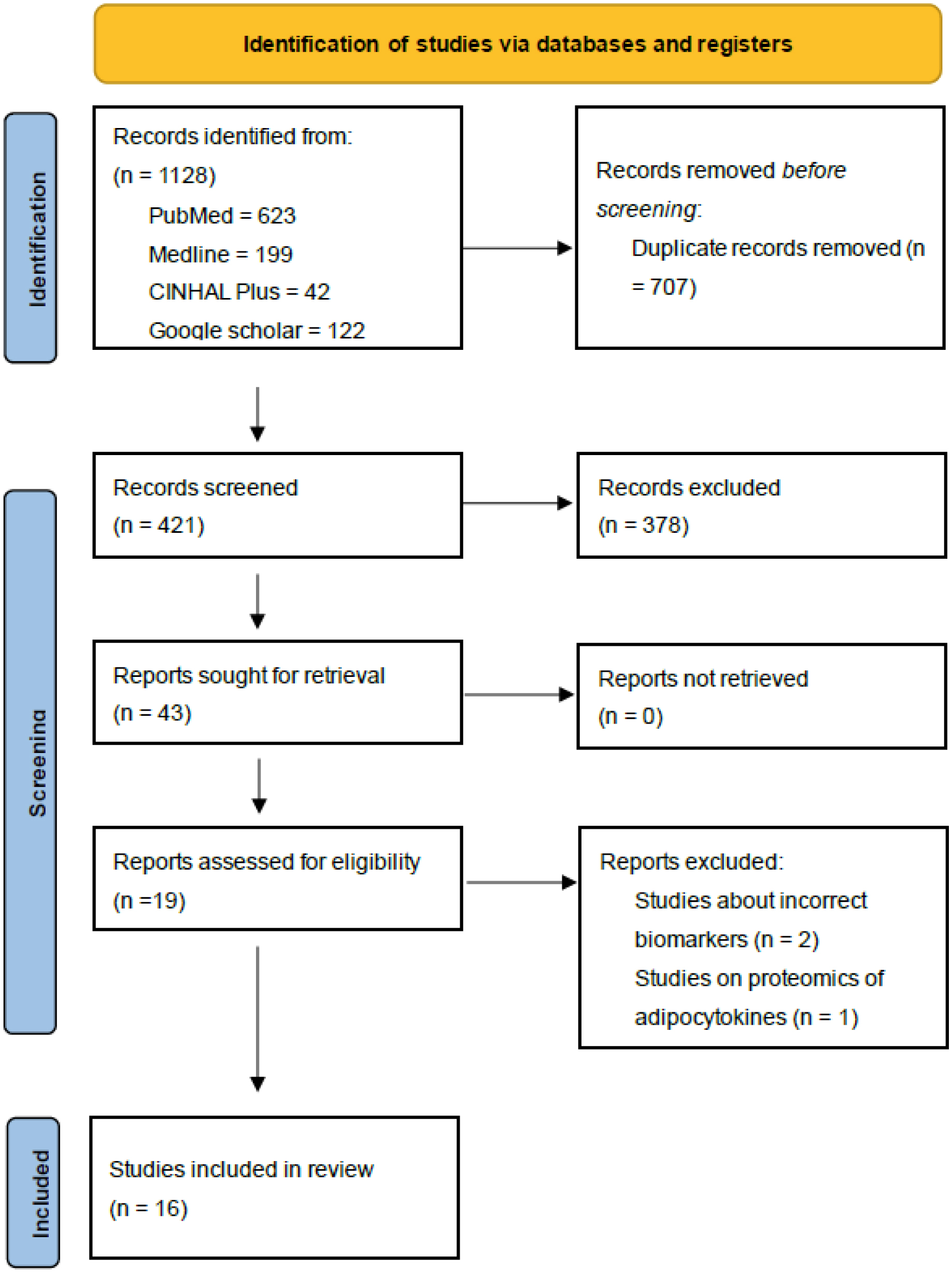
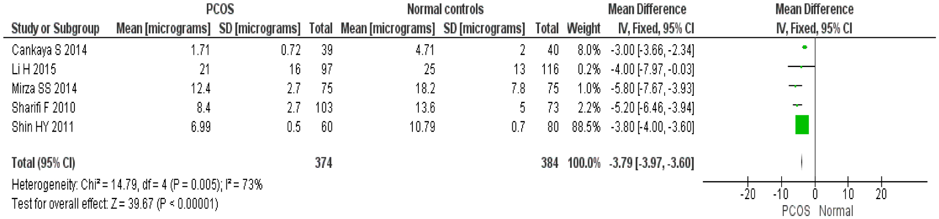
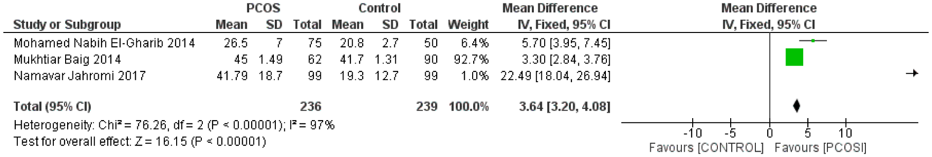
The central tenet in PCOS is predicting the development of the development of metabolic syndrome is Insulin resistance (IR). Adipocytokines are hormones produced by adipose cells that help to regulate insulin secretion and resistance in the body. This study discusses the effect of different adipocytokines and their patterns (increased or reduced) in predicting insulin resistance in obese and lean PCOS patients. A systematic review and meta-analysis were performed which identified relevant studies from 2010 to 2020. Data was analyzed using Review Manager Version (RevMan) 5.4 software. A fixed-effect model was fitted to estimate the pooled effect of adipocytokines. I² test statistics were done to test the heterogeneity of included studies. Of 17 selected studies with 1504 participants, there is considerably lower levels of adiponectin among women with PCOS as compared with healthy controls with mean difference of −3.79 (95% CI = 3.97–3.60, I² = 73%; P = 0.005). In comparison to their healthy counterparts, leptin levels were shown to be higher in women with PCOS with mean difference of 3.64 (95% CI = 3.20–4.08, I² = 97%; P = 0.00001). Leptin concentration was shown to be directly related to IR and BMI. After controlling for BMI and age-related effects, adiponectin levels appear to be lower in women with PCOS compared to non-PCOS controls but leptin levels appear to be higher. In conclusion, increased in adipocytokines such as leptin, visfatin and chemerin predict IR among both obese and lean PCOS whereas decreased levels of zinc-alpha2 glycoprotein predict IR. Adipocytokines can be potential predictive serum biomarkers of insulin resistance (IR) in PCOS.
- polycystic ovary syndrome,
- adipocytokines,
- insulin resistance
Citation: Kavitha Nagandla, Ishita Banerjee, Nafeeza Bt Hj Mohd. Ismail. Adipocytokines in polycystic ovary syndrome (PCOS): A systematic review and meta-analysis[J]. AIMS Medical Science, 2023, 10(2): 178-195. doi: 10.3934/medsci.2023016

Related Papers:

Abstract

The central tenet in PCOS is predicting the development of the development of metabolic syndrome is Insulin resistance (IR). Adipocytokines are hormones produced by adipose cells that help to regulate insulin secretion and resistance in the body. This study discusses the effect of different adipocytokines and their patterns (increased or reduced) in predicting insulin resistance in obese and lean PCOS patients. A systematic review and meta-analysis were performed which identified relevant studies from 2010 to 2020. Data was analyzed using Review Manager Version (RevMan) 5.4 software. A fixed-effect model was fitted to estimate the pooled effect of adipocytokines. I² test statistics were done to test the heterogeneity of included studies. Of 17 selected studies with 1504 participants, there is considerably lower levels of adiponectin among women with PCOS as compared with healthy controls with mean difference of −3.79 (95% CI = 3.97–3.60, I² = 73%; P = 0.005). In comparison to their healthy counterparts, leptin levels were shown to be higher in women with PCOS with mean difference of 3.64 (95% CI = 3.20–4.08, I² = 97%; P = 0.00001). Leptin concentration was shown to be directly related to IR and BMI. After controlling for BMI and age-related effects, adiponectin levels appear to be lower in women with PCOS compared to non-PCOS controls but leptin levels appear to be higher. In conclusion, increased in adipocytokines such as leptin, visfatin and chemerin predict IR among both obese and lean PCOS whereas decreased levels of zinc-alpha2 glycoprotein predict IR. Adipocytokines can be potential predictive serum biomarkers of insulin resistance (IR) in PCOS.

Use of AI tools declaration

The authors declare they have not used Artificial Intelligence (AI) tools in the creation of this article.

Conflict of interest

All authors declare no conflicts of interest in this paper.

References

[1]	Amato MC, Vesco R, Vigneri E, et al. (2015) Hyperinsulinism and polycystic ovary syndrome (PCOS): role of insulin clearance. J Endocrinol Invest 38: 1319-1326. https://doi.org/10.1007/s40618-015-0372-x
[2]	Lin K, Sun X, Wang X, et al. (2021) Circulating adipokine levels in nonobese women with polycystic ovary syndrome and in nonobese control women: A systematic review and meta-analysis. Front Endocrinol 11: 537809. https://doi.org/10.3389/fendo.2020.537809
[3]	Salley KE, Wickham EP, Cheang KI, et al. (2007) Glucose intolerance in polycystic ovary syndrome—a position statement of the Androgen Excess Society. J Clin Endocrinol Metab 92: 4546-4556. https://doi.org/10.1210/jc.2007-1549
[4]	Lee T, Rausch M (2012) Polycystic ovarian syndrome: role of imaging in diagnosis. Radiographics 32: 1643-1657. https://doi.org/10.1148/rg.326125503
[5]	Chen T, Wang F, Chu Z, et al. (2019) Serum CTRP3 levels in obese children: a potential protective adipokine of obesity, insulin sensitivity and pancreatic β cell function. Diabetes Metab Syndr Obes 12: 1923-1930. https://doi.org/10.2147/DMSO.S222066
[6]	Burghen GA, Givens JR, Kitabchi AE (1980) Correlation of hyperandrogenism with hyperinsulinism in polycystic ovarian disease. J Clin Endocrinol Metab 50: 113-116. https://doi.org/10.1210/jcem-50-1-113
[7]	DeFronzo RA, Tobin JD, Andres R (1979) Glucose clamp technique: a method for quantifying insulin secretion and resistance. Am J Physiol 237: E214-E223. https://doi.org/10.1152/ajpendo.1979.237.3.E214
[8]	Chen H, Sullivan G, Quon MJ (2005) Assessing the predictive accuracy of QUICKI as a surrogate index for insulin sensitivity using a calibration model. Diabetes 54: 1914-1925. https://doi.org/10.2337/diabetes.54.7.1914
[9]	Matthews D, Hosker J, Rudenski A, et al. (1985) Homeostasis model assessment: insulin resistance and beta-cell function from fasting plasma glucose and insulin concentrations in man. Diabetologia 28: 412-419. https://doi.org/10.1007/BF00280883
[10]	Polak K, Czyzyk A, Simoncini T, et al. (2016) New markers of insulin resistance in polycystic ovary syndrome. J Endocrinol Invest 40: 1-8. https://doi.org/10.1007/s40618-016-0523-8
[11]	Parrettini S, Cavallo M, Gaggia F, et al. (2020) Adipokines: a rainbow of proteins with metabolic and endocrine functions. Protein Pept Lett 27: 1204-1230. https://doi.org/10.2174/0929866527666200505214555
[12]	Wu H, Ballantyne C (2020) Metabolic inflammation and insulin resistance in obesity. Circ Res 126: 1549-1564. https://doi.org/10.1161/CIRCRESAHA.119.315896
[13]	Klok M, Jakobsdottir S, Drent M (2007) The role of leptin and ghrelin in the regulation of food intake and body weight in humans: a review. Obes Rev 8: 21-34. https://doi.org/10.1111/j.1467-789X.2006.00270.x
[14]	Semple R, Cochran E, Soos M, et al. (2008) Plasma adiponectin as a marker of insulin receptor dysfunction: clinical utility in severe insulin resistance. Diabetes Care 31: 977-979. https://doi.org/10.2337/dc07-2194
[15]	Fuke Y, Fujita T, Satomura A, et al. (2010) Alterations of insulin resistance and the serum adiponectin level in patients with type 2 diabetes mellitus under the usual antihypertensive dosage of telmisartan treatment. Diabetes Technol Ther 12: 393-398. https://doi.org/10.1089/dia.2009.0126
[16]	Meilleur K, Doumatey A, Huang H, et al. (2010) Circulating adiponectin is associated with obesity and serum lipids in West Africans. J Clin Endocrinol Metab 95: 3517-3521. https://doi.org/10.1210/jc.2009-2765
[17]	Brabant G, Müller G, Horn R, et al. (2005) Hepatic leptin signaling in obesity. FASEB J 19: 1048-1050. https://doi.org/10.1096/fj.04-2846fje
[18]	Ottawa Hospital Research Institute, The Newcastle-Ottawa Scale (NOS) for assessing the quality of nonrandomised studies in meta-analyses. Canada Ottawa Hospital Research Institute, 2021. Available from: http://www.ohri.ca/programs/clinical_epidemiology/oxford.asp.
[19]	Liu S, Hu W, He Y, et al. (2020) Serum Fetuin—A levels are increased and associated with insulin resistance in women with polycystic ovary syndrome. BMC Endocr Disord 20: 67. https://doi.org/10.1186/s12902-020-0538-1
[20]	Kort D, Kostolias A, Sullivan C, et al. (2015) Chemerin as a marker of body fat and insulin resistance in women with polycystic ovary syndrome. Gynecol Endocrinol 31: 152-155. https://doi.org/10.3109/09513590.2014.968547
[21]	Bannigida D, Nayak S, Vijayaragavan R (2020) Serum visfatin and adiponectin—markers in women with polycystic ovarian syndrome. Arch Physiol Biochem 126: 283-286. https://doi.org/10.1080/13813455.2018.1518987
[22]	Fouani F, Fadaei R, Moradi N, et al. (2020) Circulating levels of Meteorin-like protein in polycystic ovary syndrome: A case-control study. PLoS One 15: e0231943. https://doi.org/10.1371/journal.pone.0231943
[23]	Tang C, Li X, Tang S, et al. (2020) Association between circulating zinc-α2-glycoprotein levels and the different phenotypes of polycystic ovary syndrome. Endocr J 67: 249-255. https://doi.org/10.1507/endocrj.EJ18-0506
[24]	Shin H, Lee D, Lee J (2011) Adiponectin in women with polycystic ovary syndrome. Korean J Fam Med 32: 243-248. https://doi.org/10.4082/kjfm.2011.32.4.243
[25]	Saklayen M (2018) The global epidemic of the metabolic syndrome. Curr Hypertens Rep 20: 12. https://doi.org/10.1007/s11906-018-0812-z
[26]	DerSimonian R, Laird N (2015) Meta-analysis in clinical trials revisited. Contemp Clin Trials 45: 139-145. https://doi.org/10.1016/j.cct.2015.09.002
[27]	Gözüküçük M, Yarcı Gürsoy A, Destegül E, et al. (2020) Adiponectin and leptin levels in normal weight women with polycystic ovary syndrome. Horm Mol Biol Clin Investig 41. https://doi.org/10.1515/hmbci-2020-0016
[28]	Yildizhan R, Ilhan G, Yildizhan B, et al. (2011) Serum retinol-binding protein 4, leptin, and plasma asymmetric dimethylarginine levels in obese and nonobese young women with polycystic ovary syndrome. Fertil Steril 96: 246-250. https://doi.org/10.1016/j.fertnstert.2011.04.073
[29]	Yang S, Wang Q, Huang W, et al. (2016) Are serum chemerin levels different between obese and non-obese polycystic ovary syndrome women?. Gynecol Endocrinol 32: 38-41. https://doi.org/10.3109/09513590.2015.1075501
[30]	El‑Gharib MN, Badawy TE (2014) Correlation between insulin, leptin and polycystic ovary syndrome. J Basic Clin Reprod Sci 3: 49-53. https://doi.org/10.4103/2278-960X.129281
[31]	Cankaya S, Demir B, Aksakal SE, et al. (2014) Insulin resistance and its relationship with high molecular weight adiponectin in adolescents with polycystic ovary syndrome and a maternal history of polycystic ovary syndrome. Fertil Steril 102: 826-830. https://doi.org/10.1016/j.fertnstert.2014.05.032
[32]	Sharifi F, Hajihosseini R, Mazloomi S, et al. (2010) Decreased adiponectin levels in polycystic ovary syndrome, independent of body mass index. Metab Syndr Relat Disord 8: 47-52. https://doi.org/10.1089/met.2009.0036
[33]	Li H, Chen Y, Li Y, et al. (2015) A case-control study of correlation between serum adiponectin levels and polycystic ovary syndrome. Zhonghua Fu Chan Ke Za Zhi 50: 814-818. (Article in Chinese)
[34]	Mirza SS, Shafique K, Shaikh AR, et al. (2014) Association between circulating adiponectin levels and polycystic ovarian syndrome. J Ovarian Res 7: 18. https://doi.org/10.1186/1757-2215-7-18
[35]	Jahromi NB, Dabaghmanesh MH, Parsanezhad ME, et al. (2017) Association of leptin and insulin resistance in PCOS: A case-controlled study. Int J Reprod Biomed 15: 423-428.
[36]	Baig M, Rehman R, Tariq S, et al. (2014) Serum leptin levels in polycystic ovary syndrome and its relationship with metabolic and hormonal profile in Pakistani females. Int J Endocrinol 2014: 132908. https://doi.org/10.1155/2014/132908
[37]	Gowthami P, Kiranmayi V, Rani BS, et al. (2019) Study of serum adiponectin levels in women with polycystic ovary syndrome. Indian J Obstet Gynecol Res 6: 288-292.
[38]	Barrea L, Arnone A, Annunziata G, et al. (2019) Adherence to the Mediterranean diet, dietary patterns and body composition in women with polycystic ovary syndrome (PCOS). Nutrients 11: 2278. https://doi.org/10.3390/nu11102278

Reader Comments

Your name:*

Email:*
© 2023 the Author(s), licensee AIMS Press. This is an open access article distributed under the terms of the Creative Commons Attribution License (http://creativecommons.org/licenses/by/4.0)