Citation: Masahiro Yasunaga, Shino Manabe, Masaru Furuta, Koretsugu Ogata, Yoshikatsu Koga, Hiroki Takashima, Toshirou Nishida, Yasuhiro Matsumura. Mass spectrometry imaging for early discovery and development of cancer drugs[J]. AIMS Medical Science, 2018, 5(2): 162-180. doi: 10.3934/medsci.2018.2.162
[1] | Wai Yuen Chan . Simultaneous blow-up of the solution for a singular parabolic system with concentrated sources. AIMS Mathematics, 2024, 9(3): 6951-6963. doi: 10.3934/math.2024339 |
[2] | Varadharaj Dinakar, Natesan Barani Balan, Krishnan Balachandran . Identification of Source Terms in a Coupled Age-structured Population Model with Discontinuous Diffusion Coefficients. AIMS Mathematics, 2017, 2(1): 81-95. doi: 10.3934/Math.2017.1.81 |
[3] | Saleh Almuthaybiri, Tarek Saanouni . On coupled non-linear Schrödinger systems with singular source term. AIMS Mathematics, 2024, 9(10): 27871-27895. doi: 10.3934/math.20241353 |
[4] | Zihan Cai, Yan Liu, Baiping Ouyang . Decay properties for evolution-parabolic coupled systems related to thermoelastic plate equations. AIMS Mathematics, 2022, 7(1): 260-275. doi: 10.3934/math.2022017 |
[5] | Nataliya Gol’dman . Nonlinear boundary value problems for a parabolic equation with an unknown source function. AIMS Mathematics, 2019, 4(5): 1508-1522. doi: 10.3934/math.2019.5.1508 |
[6] | Dengming Liu, Luo Yang . Extinction behavior for a parabolic $ p $-Laplacian equation with gradient source and singular potential. AIMS Mathematics, 2022, 7(1): 915-924. doi: 10.3934/math.2022054 |
[7] | Jincheng Shi, Yan Liu . Spatial decay estimates for the coupled system of wave-plate type with thermal effect. AIMS Mathematics, 2025, 10(1): 338-352. doi: 10.3934/math.2025016 |
[8] | Xiaomin Wang, Zhong Bo Fang . New Fujita type results for quasilinear parabolic differential inequalities with gradient dissipation terms. AIMS Mathematics, 2021, 6(10): 11482-11493. doi: 10.3934/math.2021665 |
[9] | Adel M. Al-Mahdi, Mohammad M. Al-Gharabli, Nasser-Eddine Tatar . On a nonlinear system of plate equations with variable exponent nonlinearity and logarithmic source terms: Existence and stability results. AIMS Mathematics, 2023, 8(9): 19971-19992. doi: 10.3934/math.20231018 |
[10] | Najmeddine Attia, Amal Mahjoub . On the vectorial multifractal analysis in a metric space. AIMS Mathematics, 2023, 8(10): 23548-23565. doi: 10.3934/math.20231197 |
Let $ a $ and $ b $ be positive real numbers, $ c $ be a positive constant, $ x_{0} $ be a fixed point in a $ n $-dimensional space $ \mathbb{R} ^{n} $ with $ n = 1, \ 2, ... $, and $ B_{1}\left(x_{0}\right) $ be a $ n $ -dimensional open ball with the center $ x_{0} $ and radius $ 1 $ such that $ B_{1}\left(x_{0}\right) = \left\{ x\in \mathbb{R} ^{n}:\left\vert \left\vert x-x_{0}\right\vert \right\vert < 1\right\} $ where $ \left\vert \left\vert x-x_{0}\right\vert \right\vert $ represents the Euclidean distance between $ x $ and $ x_{0} $. We also let $ \overline{ B_{1}\left(x_{0}\right) } $ and $ \partial B_{1}\left(x_{0}\right) $ denote the closure and boundary of $ B_{1}\left(x_{0}\right) $, respectively. Let $ L $ be the parabolic operator such that $ Lu = u_{t}-\Delta u $. In this paper, we deal with the quenching problem of a coupled semilinear parabolic system with nonlinear singular localized sources at $ x_{0} $. This problem is described below:
$ \begin{equation} \left\{ \begin{array}{c} Lu\left( x, t\right) = af\left( v\left( x_{0}, t\right) \right) \text{ for }~~ x\in B_{1}\left( x_{0}\right) \text{ and }~~t > 0, \\ Lv\left( x, t\right) = bg\left( u\left( x_{0}, t\right) \right) \text{ for }~~ x\in B_{1}\left( x_{0}\right) \text{ and }~~t > 0, \end{array} \right. \end{equation} $ | (1.1) |
$ \begin{equation} \left\{ \begin{array}{c} u\left( x, 0\right) = 0\text{ for }~~x\in \overline{B_{1}\left( x_{0}\right) }, \text{ }u\left( x, t\right) = 0\text{ for }~~x\in \partial B_{1}\left( x_{0}\right) \text{ and }~~t > 0, \\ v\left( x, 0\right) = 0\text{ for }~~x\in \overline{B_{1}\left( x_{0}\right) }, \text{ }v\left( x, t\right) = 0\text{ for }~~x\in \partial B_{1}\left( x_{0}\right) \text{ and }~~t > 0. \end{array} \right. \end{equation} $ | (1.2) |
In the problem (1.1)-(1.2), we assume that the source functions $ f $ and $ g $ are differentiable over the interval $ \left[0, c\right) $ and satisfy the following hypotheses:
(H$ _{1} $) $ f > 0 $, $ f^{\prime } > 0 $, $ f^{\prime \prime } > 0 $, $ g > 0 $, $ g^{\prime } > 0 $, $ g^{\prime \prime } > 0 $;
(H$ _{2} $) both $ f $ and $ g $ being unbounded when $ u $ and $ v $ tend to $ c $, that is, $ f\left(v\right) \rightarrow \infty $ when $ v\rightarrow c^{-} $ (that is, $ v $ approaches $ c $ from the left) and $ g\left(u\right) \rightarrow \infty $ when $ u\rightarrow c^{-} $.
The problem (1.1)-(1.2) describes the instabilities in some dynamic systems of certain reactions that have localized electrodes immersed in a bulk medium at the point $ x_{0} $, see [1,12]. Li and Wang [10] used the equation (1.1) to explore a thermal ignition driven by the temperature at a single point. Chadam et al. [2] examined the blow-up set of solutions.
The quenching problem is able to illustrate the polarization phenomena in ionic conductors and the phase transition between liquids and solids, see [11]. We say that the solution $ \left(u, v\right) $ quenches at a point in $ \overline{B_{1}\left(x_{0}\right) } $ if there exists a finite time $ T\ \left(>0\right) $ such that
$ \max \{u\left( x, t\right) :x\in \overline{B_{1}\left( x_{0}\right) } \}\rightarrow c^{-}\text{ and }~~\max \{v\left( x, t\right) :x\in \overline{ B_{1}\left( x_{0}\right) }\}\rightarrow c^{-}\text{ as }t\rightarrow {T}^{-}, $ |
where $ t\rightarrow T^{-} $ represents $ t $ approaching $ T $ from the left. $ T $ is called the quenching time. Quenching and blow-up problems are related. Under some transformations, quenching problems are able to change to blow-up problems, see [5,6].
Ji et al. [7] studied simultaneous and non-simultaneous quenching of one-dimensional coupled system with the singular nonlinear reaction sources on the boundary. They used this model to describe heat propagations between two different materials. The multi-dimensional quenching problem of coupled semilinear parabolic systems describes non-Newtonian filtration systems incorporated with the effect of singular nonlinear reaction sources inside the domain, see Jia et al. [8]. Their model is
$ \begin{eqnarray*} Lu\left( x, t\right) & = &\left( 1-u\left( x, t\right) \right) ^{-p_{1}}+\left( 1-v\left( x, t\right) \right) ^{-q_{1}}, \ x\in \Omega , \ t > 0, \\ Lv\left( x, t\right) & = &\left( 1-u\left( x, t\right) \right) ^{-p_{2}}+\left( 1-v\left( x, t\right) \right) ^{-q_{2}}, \ x\in \Omega , \ t > 0, \\ u\left( x, 0\right) & = &u_{0}\left( x\right) , \ v\left( x, 0\right) = v_{0}\left( x\right) , \ x\in \bar{\Omega}, \\ u\left( x, t\right) & = &0, \ v\left( x, t\right) = 0, \ x\in \partial \Omega , \ t > 0, \end{eqnarray*} $ |
where $ p_{1} $, $ p_{2} $, $ q_{1} $, and $ q_{2} $ are positive real numbers, and $ \Omega $ is a bounded domain in $ \mathbb{R} ^{n} $. When $ \Omega = B_{R}\left(x_{0}\right) $, they proved that the solution $ \left(u, v\right) $ quenches simultaneously if $ p_{2}\geq p_{1}+1 $ and $ q_{1}\geq q_{2}+1 $. Depending on the initial data $ u_{0} $ and $ v_{0} $, they also showed that both simultaneous and non-simultaneous quenching may occur when $ p_{2} < p_{1}+1 $ and $ q_{1} < q_{2}+1 $. Zheng and Wang [16] studied simultaneous and non-simultaneous quenching for the coupled system: $ Lu = v^{-p} $, $ Lv = u^{-q} $ in $ B_{R}\left(x_{0}\right) \times \left(0, T\right) $ subject to the Dirichlet boundary condition. When $ \Omega $ is a square domain in $ \mathbb{R} ^{2} $, Chan [3] studied the simultaneous quenching for the coupled system: $ Lu = a/\left(1-v\left(0, 0, t\right) \right) $, $ Lv = b/\left(1-u\left(0, 0, t\right) \right) $ in $ \Omega \times \left(0, T\right) $ with the homogeneous first boundary condition. He also computed an approximated critical value of $ a $ and $ b $ by a numerical method.
The main goals of this paper are to study (a) simultaneous quenching and (b) non-simultaneous quenching of the solution $ \left(u, v\right) $ under some conditions on $ \int_{0}^{c}f\left(\omega \right) d\omega $ and $ \int_{0}^{c}g\left(\omega \right) d\omega $. In this article, simultaneous quenching means that the maximum of $ u $ and $ v $\tends to $ c $ in the same finite time. Non-simultaneous quenching means that either the maximum of $ u $ or $ v $ tends to $ c $\ in a finite time, but the other remains bounded by $ c $. We are going to study cases (a) and (b) of the problem (1.1)-(1.2) when these two integrals are either infinite or finite. Without loss of generality, let us assume $ x_{0} $ being the origin $ 0 $. The problem (1.1)-(1.2) becomes
$ \begin{equation} \left\{ \begin{array}{c} Lu = af\left( v\left( 0, t\right) \right) \text{ in }B_{1}\left( 0\right) \times \left( 0, T\right) , \\ Lv = bg\left( u\left( 0, t\right) \right) \text{ in }B_{1}\left( 0\right) \times \left( 0, T\right) , \end{array} \right. \end{equation} $ | (1.3) |
$ \begin{equation} \left\{ \begin{array}{c} u\left( x, 0\right) = 0\text{ for }~~x\in \overline{B_{1}\left( 0\right) }, \text{ }u\left( x, t\right) = 0\text{ for }~~\left( x, t\right) \in \partial B_{1}\left( 0\right) \times \left( 0, T\right) , \\ v\left( x, 0\right) = 0\text{ for }~~x\in \overline{B_{1}\left( 0\right) }, \text{ }v\left( x, t\right) = 0\text{ for }~~\left( x, t\right) \in \partial B_{1}\left( 0\right) \times \left( 0, T\right) . \end{array} \right. \end{equation} $ | (1.4) |
Similar consideration is also available in [4,8,16]. In section 2, we provide some properties of the solution $ \left(u, v\right) $. The results of simultaneous and non-simultaneous quenching are going to illustrate in section 3.
In this section, we are going to show some properties of the solution $ \left(u, v\right) $. One of the main results is to prove that $ u $ and $ v $ attain their maximum at $ x = 0 $, and they both quench only at $ x = 0 $. In the sequel, we assume that $ k_{j} $ are positive constants for $ j = 1, \ 2, ..., \ 19. $ We also let $ Y\left(x, t\right) $ and $ Z\left(x, t\right) $ be nontrivial and nonnegative bounded functions on $ \overline{B_{1}\left(0\right) }\times \left[0, \infty \right) $. Here is the comparison theorem.
Lemma 2.1. Assume that $ \left(u, v\right) $ is the solution to the problem below:
$ \left\{ \begin{array}{c} Lu\geq Y\left( x, t\right) v\left( 0, t\right) ~~{ in }~~ B_{1}\left( 0\right) \times \left( 0, T\right) , \\ Lv\geq Z\left( x, t\right) u\left( 0, t\right) ~~{ in }~~B_{1}\left( 0\right) \times \left( 0, T\right) , \end{array} \right. $ |
$ \left\{ \begin{array}{c} u\left( x, 0\right) = 0~~for~~x\in \overline{B_{1}\left( 0\right) }, u\left( x, t\right) = 0~~for~~\left( x, t\right) \in \partial B_{1}\left( 0\right) \times \left( 0, T\right) , \\ v\left( x, 0\right) = 0~~for~~x\in \overline{B_{1}\left( 0\right) }, v\left( x, t\right) = 0~~for~~\left( x, t\right) \in \partial B_{1}\left( 0\right) \times \left( 0, T\right) , \end{array} \right. $ |
then $ u\left(x, t\right) \geq 0 $ and $ v\left(x, t\right) \geq 0 $ on $ \overline{B_{1}\left(0\right) }\times \left[0, T\right) $.
Proof. Let $ \varepsilon $ be a positive real number, and
$ \begin{eqnarray*} \Phi \left( x, t\right) & = &u\left( x, t\right) +\varepsilon \hat{\phi} _{1}\left( x\right) e^{\gamma t}, \\ \Psi \left( x, t\right) & = &v\left( x, t\right) +\varepsilon \hat{\phi} _{1}\left( x\right) e^{\gamma t}, \end{eqnarray*} $ |
where $ \gamma $ is a positive real number to be determined and $ \hat{\phi} _{1} $ is the first eigenfunction of the following eigenvalue problem:
$ \Delta \hat{\phi}+\lambda \hat{\phi} = 0\text{ in }B_{1}\left( 0\right) \text{ and }~~\frac{\partial \hat{\phi}}{\partial \nu }+\hat{\phi} = 0\text{ on } \partial B_{1}\left( 0\right) , $ |
where $ \partial /\partial \nu $ is the outward normal derivative on $ \partial B_{1}\left(0\right) $. Let $ \hat{\lambda}_{1} $ be the corresponding eigenvalue. By Theorem 3.1.2 of [13], $ \hat{\phi}_{1} $ exists and $ \hat{\phi}_{1} > 0 $ on $ \overline{B_{1}\left(0\right) } $ and $ \hat{\lambda}_{1} > 0 $. Based on the construction, we know that $ \Phi \left(x, 0\right) > 0 $ and $ \Psi \left(x, 0\right) > 0 $ on $ \overline{B_{1}\left(0\right) } $. By a direct calculation, we obtain the inequality below
$ \begin{eqnarray*} &&L\Phi -Y\Psi \left( 0, t\right) \\ & = &u_{t}+\varepsilon \gamma \hat{\phi}_{1}e^{\gamma t}-\left( \Delta u+\varepsilon \Delta \hat{\phi}_{1}e^{\gamma t}\right) -Y\left( v\left( 0, t\right) +\varepsilon \hat{\phi}_{1}\left( 0\right) e^{\gamma t}\right) \\ &\geq &\varepsilon e^{\gamma t}\left( \gamma \hat{\phi}_{1}+\hat{\lambda}_{1} \hat{\phi}_{1}-Y\hat{\phi}_{1}\left( 0\right) \right) . \end{eqnarray*} $ |
Since $ \hat{\phi}_{1} > 0 $ on $ \overline{B_{1}\left(0\right) } $, $ Y $ is nonnegative and bounded, and $ \hat{\lambda}_{1} > 0 $, we are able to choose $ \gamma $ such that $ \gamma > Y\hat{\phi}_{1}\left(0\right) /\hat{\phi}_{1}- \hat{\lambda}_{1} $ in $ B_{1}\left(0\right) $. Thus,
$ L\Phi -Y\Psi \left( 0, t\right) > 0\text{ in }B_{1}\left( 0\right) \times \left( 0, T\right) . $ |
Suppose $ \Phi \left(x, t\right) \leq 0 $ somewhere in $ B_{1}\left(0\right) \times \left(0, T\right) $. Then, the set $ \left\{ t:\Phi \left(x, t\right) \leq 0\text{ for some }x\in B_{1}\left(0\right) \right\} $ is non-empty. Let $ \tilde{t} $ denote the infimum of this set. Then, $ 0 < \tilde{t} < T $ because $ \Phi \left(x, 0\right) > 0 $ on $ \overline{B_{1}\left(0\right) } $. Thus, there exists some point $ x_{1}\in B_{1}\left(0\right) $ such that $ \Phi \left(x_{1}, \tilde{t}\right) = 0 $ and $ \Phi _{t}\left(x_{1}, \tilde{t} \right) \leq 0 $. On the other hand, $ \Phi $ attains its local minimum at $ \left(x_{1}, \tilde{t}\right) $. Then, $ \Delta \Phi \left(x_{1}, \tilde{t} \right) \geq 0 $. Let us consider $ t = \tilde{t} $, we get
$ \begin{equation} \Phi _{t}\left( x_{1}, \tilde{t}\right) -Y\left( x_{1}, \tilde{t}\right) \Psi \left( 0, \tilde{t}\right) \geq L\Phi \left( x_{1}, \tilde{t}\right) -Y\left( x_{1}, \tilde{t}\right) \Psi \left( 0, \tilde{t}\right) > 0. \end{equation} $ | (2.1) |
Follow a similar argument, if we assume that $ \Psi \left(x, t\right) \leq 0 $ somewhere in $ B_{1}\left(0\right) \times \left(0, T\right) $, then there exist some $ \hat{t}\in \left(0, T\right) $ and $ x_{2}\in B_{1}\left(0\right) $ such that $ \Psi \left(x_{2}, \hat{t}\right) = 0 $, $ \Psi _{t}\left(x_{2}, \hat{t}\right) \leq 0 $, and $ \Psi $ attains its local minimum at $ \left(x_{2}, \hat{t}\right) $. Then, at $ t = \hat{t} $
$ \begin{equation} \Psi _{t}\left( x_{2}, \hat{t}\right) -Z\left( x_{2}, \hat{t}\right) \Phi \left( 0, \hat{t}\right) \geq L\Psi \left( x_{2}, \hat{t}\right) -Z\left( x_{2}, \hat{t}\right) \Phi \left( 0, \hat{t}\right) > 0. \end{equation} $ | (2.2) |
Let us assume that $ \hat{t} < \tilde{t} $. As $ \Phi $ attains its local minimum at $ \left(x_{1}, \tilde{t}\right) $, we have $ \Phi \left(0, \hat{t}\right) > 0 $. From the expression (2.2) and $ Z $ is nonnegative and bounded, we have the inequality below:
$ 0\geq \Psi _{t}\left( x_{2}, \hat{t}\right) \geq \Psi _{t}\left( x_{2}, \hat{t} \right) -Z\left( x_{2}, \hat{t}\right) \Phi \left( 0, \hat{t}\right) > 0. $ |
This is a contradiction. Hence, $ \Psi \left(x, t\right) > 0 $ in $ B_{1}\left(0\right) \times \left(0, T\right) $. Then by (2.1), we show that $ \Phi \left(x, t\right) > 0 $ in $ B_{1}\left(0\right) \times \left(0, T\right) $. Through a similar calculation, we obtain the same result when $ \hat{t}\geq \tilde{t} $. Let $ \varepsilon \rightarrow 0 $, we have $ u\left(x, t\right) \geq 0 $ and $ v\left(x, t\right) \geq 0 $ in $ B_{1}\left(0\right) \times \left(0, T\right) $. Following the homogeneous initial-boundary conditions, we conclude that $ u $ and $ v $ are non-negative on $ \overline{B_{1}\left(0\right) }\times \left[0, T\right) $. The proof is complete.
By Lemma 2.1, $ \left(0, 0\right) $ is a lower solution of the problem (1.3)-(1.4). On the other side, $ u < c $ and $ v < c $ on $ \overline{B_{1}\left(0\right) }\times \left[0, T\right) $. Since $ u $ and $ v $ stop to exist for $ u\geq c $ and $ v\geq c $, it follows from Theorem 2.1 of [2] that the problem (1.3)-(1.4) has the unique classical solution $ \left(u, v\right) \in C\left(\overline{B_{1}\left(0\right) }\times \left[0, T\right) \right) \cap C^{2+\alpha, 1+\alpha /2}\left(B_{1}\left(0\right) \times \left[0, T\right) \right) $ for some $ \alpha \in \left(0, 1\right) $ such that $ 0\leq u < c $ and $ 0\leq v < c $ on $ \overline{B_{1}\left(0\right) }\times \left[0, T\right) $. As $ f $ and $ g $ are differentiable, it follows from Theorem 8.9.2 of Pao [13] that the solution $ \left(u, v\right) $ exists either in a finite time or globally.
Based on the result of Lemma 2.1, we prove $ u_{t} $ and $ v_{t} $ being positive over the domain.
Lemma 2.2. The solution $ \left(u, v\right) $ has the properties: (i) $ u_{t}\geq 0 $ and $ v_{t}\geq 0 $ on $ \overline{B_{1}\left(0\right) }\times \left[0, T\right) $, and (ii) $ u_{t} > 0 $ and $ v_{t} > 0 $ in $ B_{1}\left(0\right) \times \left(0, T\right) $.
Proof. (i) For $ \theta _{1} > 0 $, let us consider the first equation of the problem (1.3) at $ t+\theta _{1} $. We have $ Lu\left(x, t+\theta _{1}\right) = af\left(v\left(0, t+\theta _{1}\right) \right) $ in $ B_{1}\left(0\right) \times \left(0, T-\theta _{1}\right) $. Subtract the first equation of the problem (1.3) from this equation, and based on the mean value theorem, there exists some $ \zeta _{1} $ where $ \zeta _{1} $ is between $ v\left(0, t+\theta _{1}\right) $ and $ v\left(0, t\right) $ such that
$ Lu\left( x, t+\theta _{1}\right) -Lu\left( x, t\right) = af^{\prime }\left( \zeta _{1}\right) \left[ v\left( 0, t+\theta _{1}\right) -v\left( 0, t\right) \right] \text{ in }B_{1}\left( 0\right) \times \left( 0, T-\theta _{1}\right) . $ |
Since $ u\geq 0 $ on $ \overline{B_{1}\left(0\right) }\times \left[0, T\right) $, we have $ u\left(x, \theta _{1}\right) -u\left(x, 0\right) \geq 0 $ for $ x\in \overline{B_{1}\left(0\right) } $. From the boundary condition, $ u\left(x, t+\theta _{1}\right) -u\left(x, t\right) = 0 $ for $ x\in \partial B_{1}\left(0\right) $ and $ t > 0 $. By Lemma 2.1, $ \left(u(x, t+\theta _{1})-u(x, t)\right) /\theta _{1}\geq 0 $ on $ \overline{B_{1}\left(0\right) } \times \left[0, T-\theta _{1}\right) $. As $ \theta _{1}\rightarrow 0^{+} $, $ u_{t}\geq 0 $ on $ \overline{B_{1}\left(0\right) }\times \left[0, T\right) $. Similarly, we obtain $ v_{t}\geq 0 $ on $ \overline{B_{1}\left(0\right) } \times \left[0, T\right) $.
(ii) To show that $ u_{t} $ is positive, we differentiate the first equation of the problem (1.3) with respect to $ t $ to get
$ Lu_{t} = af^{\prime }\left( v\left( 0, t\right) \right) v_{t}\left( 0, t\right) \text{ in }B_{1}\left( 0\right) \times \left( 0, T\right) . $ |
From (i), we know $ v_{t}\geq 0 $ on $ \overline{B_{1}\left(0\right) }\times \left[0, T\right) $. By (H$ _{1} $) (see section 1) and the strong maximum principle, we have $ u_{t} > 0 $ in $ B_{1}\left(0\right) \times \left(0, T\right) $. We follow the similar procedure to conclude $ v_{t} > 0 $ in $ B_{1}\left(0\right) \times \left(0, T\right) $.
By the symmetry of $ B_{1}\left(0\right) $, we represent the problem (1.3)-(1.4) in the polar coordinate system
$ \begin{equation} \left\{ \begin{array}{c} u_{t}\left( r, t\right) -u_{rr}\left( r, t\right) -\dfrac{n-1}{r}u_{r}\left( r, t\right) = af\left( v\left( 0, t\right) \right) \text{ in }\left( 0, 1\right) \times \left( 0, T\right) , \\ v_{t}\left( r, t\right) -v_{rr}\left( r, t\right) -\dfrac{n-1}{r}v_{r}\left( r, t\right) = bg\left( u\left( 0, t\right) \right) \text{ in }\left( 0, 1\right) \times \left( 0, T\right) , \\ u\left( r, 0\right) = 0\text{ for }~~r\in \left[ 0, 1\right] \text{, }\ u_{r}\left( 0, t\right) = 0\text{ and }~~u\left( 1, t\right) = 0\text{ for }~~t\in \left( 0, T\right) , \\ v\left( r, 0\right) = 0\text{ for }~~r\in \left[ 0, 1\right] \text{, }\ v_{r}\left( 0, t\right) = 0\text{ and }~~v\left( 1, t\right) = 0\text{ for }~~t\in \left( 0, T\right) . \end{array} \right. \end{equation} $ | (2.3) |
Lemma 2.3. The solution $ \left(u, v\right) $ to the problem (2.4) attains its maximum at $ r = 0 $ for $ t\in \left(0, T\right) $.
Proof. It is noticed that the solution to the problem (2.4) is radial symmetric with respect to $ r = 0 $. To show $ u $ and $ v $ attaining their maximum at $ r = 0 $, we are going to prove $ u_{r} < 0 $ and $ v_{r} < 0 $ for $ r\in \left(0, 1\right] $. We let $ H\left(r, t\right) = u_{r}\left(r, t\right) $. Differentiating the first equation of the problem (2.4) with respect to $ r $, we have
$ H_{t}-H_{rr}-\frac{n-1}{r}H_{r}+\frac{n-1}{r^{2}}H = 0\text{ in }\left( 0, 1\right) \times \left( 0, T\right) . $ |
At $ t = 0 $, $ H\left(r, 0\right) = 0 $ for $ r\in \lbrack 0, 1] $. By Lemma 2.2(ii), $ u_{t} > 0 $ in $ B_{1}\left(0\right) \times \left(0, T\right) $. By Hopf's Lemma, $ H\left(1, t\right) < 0 $ for $ t\in \left(0, T\right) $. Also, $ H\left(0, t\right) = u_{r}\left(0, t\right) = 0 $ for $ t\in \left[0, T\right) $. By the maximum principle [13], $ H < 0 $ for $ \left(r, t\right) \in \left(0, 1\right] \times \left(0, T\right) $. Therefore, $ u\left(0, t\right) \geq u\left(r, t\right) $ for $ \left(r, t\right) \in \left[0, 1\right] \times \left(0, T\right) $. Similarly, we prove that $ v_{r} < 0 $ for $ \left(r, t\right) \in \left(0, 1\right] \times \left(0, T\right) $. Hence, $ u $ and $ v $ achieve their maximum at $ r = 0 $ for $ t\in \left(0, T\right). $
Let $ \phi _{1} $ be the eigenfunction corresponding to the first eigenvalue $ \lambda _{1}\left(>0\right) $ of the eigenvalue problem below:
$ \Delta \phi +\lambda \phi = 0\text{ in }B_{1}\left( 0\right) \text{, }\phi = 0 \text{ on }\partial B_{1}\left( 0\right) . $ |
This eigenfunction has the properties: $ 0 < \phi _{1}\leq 1 $ in $ B_{1}\left(0\right) $ and $ \int_{B_{1}\left(0\right) }\phi _{1}dx = 1 $ [15]. Let $ k_{1} = abf^{\prime \prime }\left(0\right) g^{\prime \prime }\left(0\right) / \left[2\left(af^{\prime \prime }\left(0\right) +bg^{\prime \prime }\left(0\right) \right) \right] $ and $ k_{2} = af\left(0\right) +bg\left(0\right) $. By (H$ _{1} $), $ k_{1} $ and $ k_{2} $ are positive. We show that either $ u $ or $ v $ quenches in a finite time.
Lemma 2.4. If $ 2\sqrt{k_{1}k_{2}} > \lambda _{1} $, then either $ u $ or $ v $ quenches on $ \overline{ B_{1}\left(0\right) } $ in a finite time $ \tilde{T} $.
Proof. By Lemma 2.3, $ u\left(0, t\right) \geq u\left(x, t\right) $ and $ v\left(0, t\right) \geq v\left(x, t\right) $ on $ \overline{ B_{1}\left(0\right) }\times \left(0, T\right) $. Let $ \hat{u}\left(x, t\right) $ and $ \hat{v}\left(x, t\right) $ be the solutions to the following auxiliary parabolic system:
$ \begin{equation} \left\{ \begin{array}{c} L\hat{u} = af\left( \hat{v}\left( x, t\right) \right) \text{ in }B_{1}\left( 0\right) \times \left( 0, T\right) , \\ L\hat{v} = bg(\hat{u}(x, t))\text{ in }B_{1}\left( 0\right) \times \left( 0, T\right) , \end{array} \right. \end{equation} $ | (2.4) |
$ \begin{equation} \left\{ \begin{array}{c} \hat{u}\left( x, 0\right) = 0\text{ and }~~\hat{v}\left( x, 0\right) = 0\text{ on } \overline{B_{1}\left( 0\right) }, \\ \hat{u}\left( x, t\right) = 0\text{ and }~~\hat{v}\left( x, t\right) = 0\text{ on } \partial B_{1}\left( 0\right) \times \left( 0, T\right) . \end{array} \right. \end{equation} $ | (2.5) |
By the comparison theorem [13], $ \hat{u}\left(x, t\right) \geq 0 $ and $ \hat{v}\left(x, t\right) \geq 0 $ on $ \overline{B_{1}\left(0\right) }\times \left(0, T\right) $. Further, $ u-\hat{u} $ and $ v-\hat{v} $ satisfy the expression below:
$ \begin{eqnarray*} L\left( u-\hat{u}\right) & = &af\left( v\left( 0, t\right) \right) -af\left( \hat{v}\left( x, t\right) \right) \geq af\left( v\left( x, t\right) \right) -af\left( \hat{v}\left( x, t\right) \right) , \\ L\left( v-\hat{v}\right) & = &bg(u(0, t))-bg(\hat{u}(x, t))\geq bg(u(x, t))-bg( \hat{u}(x, t)). \end{eqnarray*} $ |
By $ u-\hat{u} = 0 $ and $ v-\hat{v} = 0 $ on $ \overline{B_{1}\left(0\right) } $ and $ \partial B_{1}\left(0\right) \times \left(0, T\right) $, and the comparison theorem, we have $ u\geq \hat{u} $ and $ v\geq \hat{v} $ on $ \overline{B_{1}\left(0\right) }\times \left(0, T\right) $. It suffices to prove either $ \hat{u} $ or $ \hat{v} $ to quench over $ \overline{B_{1}\left(0\right) } $ in a finite time. Multiplying $ \phi _{1} $ on both sides of (2.5) and integrating expressions over the domain $ B_{1}\left(0\right) $, we obtain
$ \int_{B_{1}\left( 0\right) }\hat{u}_{t}\phi _{1}dx-\int_{B_{1}\left( 0\right) }\Delta \hat{u}\phi _{1}dx = a\int_{B_{1}\left( 0\right) }\phi _{1}f\left( \hat{v}\left( x, t\right) \right) dx, $ |
$ \int_{B_{1}\left( 0\right) }\hat{v}_{t}\phi _{1}dx-\int_{B_{1}\left( 0\right) }\Delta \hat{v}\phi _{1}dx = b\int_{B_{1}\left( 0\right) }\phi _{1}g\left( \hat{u}\left( x, t\right) \right) dx. $ |
Using the Green's second identity and (2.6), it gives
$ \left( \int_{B_{1}\left( 0\right) }\hat{u}\phi _{1}dx\right) _{t} = -\lambda _{1}\int_{B_{1}\left( 0\right) }\hat{u}\phi _{1}dx+a\int_{B_{1}\left( 0\right) }\phi _{1}f\left( \hat{v}\right) dx, $ |
$ \left( \int_{B_{1}\left( 0\right) }\hat{v}\phi _{1}dx\right) _{t} = -\lambda _{1}\int_{B_{1}\left( 0\right) }\hat{v}\phi _{1}dx+b\int_{B_{1}\left( 0\right) }\phi _{1}g\left( \hat{u}\right) dx. $ |
Applying the Maclaurin's series on the functions $ f $ and $ g $, we have
$ \left( \int_{B_{1}\left( 0\right) }\hat{u}\phi _{1}dx\right) _{t}\geq -\lambda _{1}\int_{B_{1}\left( 0\right) }\hat{u}\phi _{1}dx+a\int_{B_{1}\left( 0\right) }\frac{f^{\prime \prime }\left( 0\right) }{2}\left( \hat{v}\right) ^{2}\phi _{1}dx+a\int_{B_{1}\left( 0\right) }f\left( 0\right) \phi _{1}dx, $ |
$ \left( \int_{B_{1}\left( 0\right) }\hat{v}\phi _{1}dx\right) _{t}\geq -\lambda _{1}\int_{B_{1}\left( 0\right) }\hat{v}\phi _{1}dx+b\int_{B_{1}\left( 0\right) }\frac{g^{\prime \prime }\left( 0\right) }{2}\left( \hat{u}\right) ^{2}\phi _{1}dx+b\int_{B_{1}\left( 0\right) }g\left( 0\right) \phi _{1}dx. $ |
By $ 0 < \phi _{1}\leq 1 $ in $ B_{1}\left(0\right) $ and the Jensen's inequality [15], we have
$ \begin{eqnarray*} \int_{B_{1}\left( 0\right) }\left( \hat{v}\right) ^{2}\phi _{1}dx &\geq &\int_{B_{1}\left( 0\right) }\left( \hat{v}\right) ^{2}\left( \phi _{1}\right) ^{2}dx\geq \left( \int_{B_{1}\left( 0\right) }\hat{v}\phi _{1}dx\right) ^{2}, \\ \int_{B_{1}\left( 0\right) }\left( \hat{u}\right) ^{2}\phi _{1}dx &\geq &\int_{B_{1}\left( 0\right) }\left( \hat{u}\right) ^{2}\left( \phi _{1}\right) ^{2}dx\geq \left( \int_{B_{1}\left( 0\right) }\hat{u}\phi _{1}dx\right) ^{2}. \end{eqnarray*} $ |
Let $ R\left(t\right) = \int_{B_{1}\left(0\right) }\hat{u}\phi _{1}dx $ and $ P\left(t\right) = \int_{B_{1}\left(0\right) }\hat{v}\phi _{1}dx $. From these two inequalities above, we have the following inequality:
$ \begin{equation} \frac{d}{dt}\left( P+R\right) \geq -\lambda _{1}\left( P+R\right) +\frac{ af^{\prime \prime }\left( 0\right) }{2}P^{2}+\frac{bg^{\prime \prime }\left( 0\right) }{2}R^{2}+af\left( 0\right) +bg\left( 0\right) . \end{equation} $ | (2.6) |
Then, by the inequality below:
$ \begin{eqnarray*} &&\frac{\left( \frac{af^{\prime \prime }\left( 0\right) }{2}-k_{1}\right) P^{2}+\left( \frac{bg^{\prime \prime }\left( 0\right) }{2}-k_{1}\right) R^{2} }{2} \\ &\geq &\sqrt{\left( \frac{af^{\prime \prime }\left( 0\right) }{2}+\frac{ bg^{\prime \prime }\left( 0\right) }{2}\right) \left[ \frac{abf^{\prime \prime }\left( 0\right) g^{\prime \prime }\left( 0\right) }{2\left( af^{\prime \prime }\left( 0\right) +bg^{\prime \prime }\left( 0\right) \right) }-k_{1}\right] +k_{1}^{2}}PR \\ & = &k_{1}PR, \end{eqnarray*} $ |
we obtain this expression
$ \frac{af^{\prime \prime }\left( 0\right) }{2}P^{2}+\frac{bg^{\prime \prime }\left( 0\right) }{2}R^{2}\geq k_{1}\left( P+R\right) ^{2}. $ |
Then, the differential inequality (2.7) becomes
$ \frac{d}{dt}\left( P+R\right) \geq -\lambda _{1}\left( P+R\right) +k_{1}(P+R)^{2}+k_{2}. $ |
Let $ E\left(t\right) = P\left(t\right) +R\left(t\right) $. Then, $ E\left(t\right) \geq 0 $ in $ \left[0, T\right) $ and
$ \frac{d}{dt}E\geq -\lambda _{1}E+k_{1}E^{2}+k_{2}. $ |
Using separation of variables and integrating both sides over $ \left(0, t\right) $, we obtain
$ t\leq \frac{2}{\sqrt{4k_{1}k_{2}-\lambda _{1}^{2}}}\left[ \tan ^{-1}\left( \frac{2k_{1}E\left( t\right) -\lambda _{1}}{\sqrt{4k_{1}k_{2}-\lambda _{1}^{2}}}\right) +\tan ^{-1}\left( \frac{\lambda _{1}}{\sqrt{ 4k_{1}k_{2}-\lambda _{1}^{2}}}\right) \right] . $ |
Suppose that $ E\left(t\right) $ exists for all $ t > 0 $. By the assumption $ 2 \sqrt{k_{1}k_{2}} > \lambda _{1} $, we have
$ \tan ^{-1}\left( \frac{2k_{1}E\left( t\right) -\lambda _{1}}{\sqrt{ 4k_{1}k_{2}-\lambda _{1}^{2}}}\right) \rightarrow \infty \text{ if } t\rightarrow \infty . $ |
But, $ \tan ^{-1}\left[\left(2k_{1}E\left(t\right) -\lambda _{1}\right) / \sqrt{4k_{1}k_{2}-\lambda _{1}^{2}}\right] $ is bounded above by $ \pi /2 $. This is a contradiction. It implies that $ E(t) $ ceases to exist in a finite time $ \hat{T} $. This shows that either $ P\left(t\right) $ or $ R\left(t\right) $ does not exist when $ t $ tends to $ \hat{T} $. Thus, either $ \hat{u} $ or $ \hat{v} $ quenches on $ \overline{B_{1}\left(0\right) } $ at $ \hat{T} $. Since $ u\geq \hat{u} $ and $ v\geq \hat{v} $, we then have either $ u $ or $ v $ quenches on $ \overline{B_{1}\left(0\right) } $ in a finite time $ \tilde{T} $ where $ \tilde{T}\leq \hat{T} $.
Let $ M_{1} $ and $ M_{2} $ be positive constants such that $ M_{1}/\left(2n\right) < c $ and $ M_{2}/\left(2n\right) < c $. We are going to prove the global existence of solutions when $ a $ and $ b $ are sufficiently small. Our method is to construct a global-existed upper solution of the problem (1.1)-(1.2).
Lemma 2.5. If $ a $ and $ b $ are sufficiently small, then the solution $ \left(u, v\right) $ exists globally.
Proof. It suffices to construct an upper solution which exists all time. Let $ \bar{u}\left(x\right) = M_{1}\left(1-\left\Vert x\right\Vert ^{2}\right) /\left(2n\right) $ and $ \bar{v}\left(x\right) = M_{2}\left(1-\left\Vert x\right\Vert ^{2}\right) /\left(2n\right) $. Clearly, $ 0\leq \bar{u} $, $ \bar{v} < c $ for all $ x\in \overline{B_{1}\left(0\right) } $. Let us consider the following problem:
$ \begin{array}{c} L\bar{u}-af\left( \bar{v}\left( 0\right) \right) = M_{1}-af\left( M_{2}/\left( 2n\right) \right) , \\ L\bar{v}-bg\left( \bar{u}\left( 0\right) \right) = M_{2}-bg\left( M_{1}/\left( 2n\right) \right) . \end{array} $ |
If $ a $ and $ b $ are sufficiently small, then
$ \begin{array}{c} L\bar{u}-af\left( \bar{v}\left( 0\right) \right) = M_{1}-af\left( M_{2}/\left( 2n\right) \right) \geq 0\text{ in }B_{1}\left( 0\right) \times \left( 0, \infty \right) , \\ L\bar{v}-bg\left( \bar{u}\left( 0\right) \right) = M_{2}-bg\left( M_{1}/\left( 2n\right) \right) \geq 0\text{ in }B_{1}\left( 0\right) \times \left( 0, \infty \right) . \end{array} $ |
Then, we subtract Eq (1.3) from above inequalities and by the mean value theorem to obtain
$ \begin{array}{c} L\left( \bar{u}-u\right) \geq a\left[ f\left( \bar{v}\left( 0\right) \right) -f\left( v\left( 0, t\right) \right) \right] = af^{\prime }\left( \chi _{1}\right) \left[ \bar{v}\left( 0\right) -v\left( 0, t\right) \right] \text{ in }B_{1}\left( 0\right) \times \left( 0, \infty \right) , \\ L\left( \bar{v}-v\right) \geq b\left[ g\left( \bar{u}\left( 0\right) \right) -g\left( u\left( 0, t\right) \right) \right] = bg^{\prime }\left( \chi _{2}\right) \left[ \bar{u}\left( 0\right) -u\left( 0, t\right) \right] \text{ in }B_{1}\left( 0\right) \times \left( 0, \infty \right) , \end{array} $ |
where $ \chi _{1} $ is between $ \bar{v}\left(0\right) $ and $ v\left(0, t\right) $ and $ \chi _{2} $ is between $ \bar{u}\left(0\right) $ and $ u\left(0, t\right) $. On $ \partial B_{1}\left(0\right) $, $ \bar{u}-u = 0 $ and $ \bar{v}-v = 0 $. By Lemma 2.1, $ u\left(x, t\right) \leq \bar{u}\left(x\right) $ and $ v\left(x, t\right) \leq \bar{v}\left(x\right) $ on $ \overline{B_{1}\left(0\right) }\times \left[0, \infty \right) $. Thus, the solution $ \left(u, v\right) $ exists globally. The proof is complete.
From the result of Lemma 2.3, we know that $ x = 0 $ is a quenching point of $ u $ and $ v $ if they quench. Let $ T^{\ast } $ be the supremum of the time $ T $ for which the problem (1.3)-(1.4) has the unique solution $ \left(u, v\right) $.
Theorem 2.6. If $ T^{\ast } < \infty $, then either $ u\left(0, t\right) $ or $ v\left(0, t\right) $ quenches at $ T^{\ast } $.
Proof. Suppose that both $ u $ and $ v $ do not quench at $ x = 0 $ when $ t = T^{\ast } $. Then, there exist $ k_{3} $ and $ k_{4} $ such that $ u\left(0, t\right) \leq k_{3} < c $ and $ v\left(0, t\right) \leq k_{4} < c $ for $ t\in \left[0, T^{\ast }\right] $. This shows that $ af\left(v\left(0, t\right) \right) < k_{5} $ and $ bg\left(u\left(0, t\right) \right) < k_{6} $ for $ t\in \left[0, T^{\ast }\right] $. Then, by Theorem 4.2.1 of [9], $ u $ and $ v\in C^{2+\alpha, 1+\alpha /2}\left(\overline{ B_{1}\left(0\right) }\times \lbrack 0, T^{\ast }]\right) $. This implies that there exist $ k_{7} $ and $ k_{8} $ such that $ u\left(x, t\right) \leq k_{7} < c $ and $ v\left(x, t\right) \leq k_{8} < c $ for $ \left(x, t\right) \in \overline{B_{1}\left(0\right) }\times \left[0, T^{\ast }\right] $. In order to arrive at a contradiction, we need to show that $ u $ and $ v $ can continue to exist in a longer time interval $ \left[0, T^{\ast }+t_{1}\right) $ for some positive $ t_{1} $. This can be accomplished by extending the upper bound of $ u $ and $ v $. Let us construct upper solutions $ \psi \left(x, t\right) = k_{7}h\left(t\right) $ and $ \sigma \left(x, t\right) = k_{8}i\left(t\right) $, where $ h\left(t\right) $ and $ i\left(t\right) $ are solutions to the following system:
$ \begin{eqnarray*} \frac{d}{dt}k_{7}h\left( t\right) & = &af\left( k_{8}i\left( t\right) \right) \text{ for }~~t > T^{\ast }, \ h\left( T^{\ast }\right) = 1, \\ \frac{d}{dt}k_{8}i\left( t\right) & = &bg\left( k_{7}h\left( t\right) \right) \text{ for }~~t > T^{\ast }, \ i\left( T^{\ast }\right) = 1. \end{eqnarray*} $ |
From $ af\left(k_{8}i\left(t\right) \right) > 0 $ and $ bg\left(k_{7}h\left(t\right) \right) > 0 $, this implies that $ h\left(t\right) $ and $ i\left(t\right) $ are increasing functions of $ t $. Let $ t_{1} $ be a positive real number determined by $ k_{7}h\left(T^{\ast }+t_{1}\right) = k_{9} < c $ and $ k_{8}i\left(T^{\ast }+t_{1}\right) = k_{10} < c $ for some $ k_{9}\left(>k_{7}\right) $ and $ k_{10}\left(>k_{8}\right) $. By our construction, $ \psi \left(x, t\right) = \psi \left(0, t\right) $ and $ \sigma \left(x, t\right) = \sigma \left(0, t\right) $ satisfy
$ \begin{eqnarray*} L\psi \left( x, t\right) & = &af\left( \sigma \left( 0, t\right) \right) \text{ in }B_{1}\left( 0\right) \times \left( T^{\ast }, T^{\ast }+t_{1}\right) , \\ L\sigma \left( x, t\right) & = &bg\left( \psi \left( 0, t\right) \right) \text{ in }B_{1}\left( 0\right) \times \left( T^{\ast }, T^{\ast }+t_{1}\right) , \\ \psi \left( x, T^{\ast }\right) & = &k_{7}h\left( T^{\ast }\right) \geq u\left( x, T^{\ast }\right) \text{ and }~~\sigma \left( x, T^{\ast }\right) = k_{8}i\left( T^{\ast }\right) \geq v\left( x, T^{\ast }\right) \text{ on } \overline{B_{1}\left( 0\right) }, \\ \psi \left( x, t\right) & = &k_{7}h\left( t\right) > 0\text{ and }~~\sigma \left( x, t\right) = k_{8}i\left( t\right) > 0\text{ on }\partial B_{1}\left( 0\right) \times \left( T^{\ast }, T^{\ast }+t_{1}\right) . \end{eqnarray*} $ |
By Lemma 2.1, $ \psi \left(x, t\right) \geq u\left(x, t\right) $ and $ \sigma \left(x, t\right) \geq v\left(x, t\right) $ on $ \overline{B_{1}\left(0\right) }\times \left[T^{\ast }, T^{\ast }+t_{1}\right) $. Therefore, we find the solution $ \left(u, v\right) $ to the problem (1.3)-(1.4) on $ \overline{B_{1}\left(0\right) }\times \left[T^{\ast }, T^{\ast }+t_{1}\right) $. This contradicts the definition of $ T^{\ast } $. Hence, either $ u\left(0, t\right) $ or $ v\left(0, t\right) $ quenches at $ T^{\ast } $.
Let $ y = u_{t} $ and $ z = v_{t} $. We differentiate the problem (2.4) with respect to $ t $ to obtain the following system
$ \begin{equation} \left\{ \begin{array}{c} y_{t}\left( r, t\right) -y_{rr}\left( r, t\right) -\dfrac{\left( n-1\right) }{r }y_{r}\left( r, t\right) = af^{\prime }\left( v\left( 0, t\right) \right) z\left( 0, t\right) \text{ in }\left( 0, 1\right) \times \left( 0, T\right) , \\ z_{t}\left( r, t\right) -z_{rr}\left( r, t\right) -\dfrac{\left( n-1\right) }{r }z_{r}\left( r, t\right) = ag^{\prime }\left( u\left( 0, t\right) \right) y\left( 0, t\right) \text{ in }\left( 0, 1\right) \times \left( 0, T\right) , \\ y\left( r, 0\right) \geq 0\text{ for }~~r\in \left[ 0, 1\right) \text{ and }~~ y\left( 1, 0\right) = 0\text{, }y\left( 0, t\right) > 0\text{ and }~~y\left( 1, t\right) = 0\text{ for }~~t\in \left( 0, T\right) , \\ z\left( r, 0\right) \geq 0\text{ for }~~r\in \left[ 0, 1\right) \text{ and }~~ z\left( 1, 0\right) = 0\text{, }z\left( 0, t\right) > 0\text{ and }~~z\left( 1, t\right) = 0\text{ for }~~t\in \left( 0, T\right) . \end{array} \right. \end{equation} $ | (2.7) |
The result below shows that $ u_{t}\left(r, t\right) $ and $ v_{t}\left(r, t\right) $ are decreasing functions in $ r $.
Lemma 2.7. $ u_{t}\left(r_{2}, t\right) < u_{t}\left(r_{1}, t\right) $ and $ v_{t}\left(r_{2}, t\right) < v_{t}\left(r_{1}, t\right) $ for $ 0 < r_{1} < r_{2} < 1 $ and $ t\in \left(0, T\right) $.
Proof. We differentiate the first equation of problem (2.8) with respect to $ r $ to obtain the following differential equation
$ y_{tr}-y_{rrr}-\frac{\left( n-1\right) }{r}y_{rr}+\frac{\left( n-1\right) }{ r^{2}}y_{r} = 0. $ |
For $ r\in \left[0, 1\right) $, $ u_{rt}\left(r, 0\right) $ is given by
$ u_{rt}\left( r, 0\right) = \lim\limits_{\theta _{1}\rightarrow 0}\frac{u_{r}\left( r, \theta _{1}\right) -u_{r}\left( r, 0\right) }{\theta _{1}}. $ |
Using $ u_{r}\left(r, 0\right) = 0 $ and Lemma 2.3, we have $ u_{rt}\left(r, 0\right) \leq 0 $. Thus, $ y_{r}\left(r, 0\right) \leq 0 $ for $ r\in \left[0, 1\right) $. By Lemma 2.2(i),
$ \frac{\partial y\left( 1, 0\right) }{\partial r} = \lim\limits_{\theta _{2}\rightarrow 0}\frac{y\left( 1, 0\right) -y\left( 1-\theta _{2}, 0\right) }{\theta _{2}} \leq 0. $ |
By the Hopf's lemma, $ \partial y\left(1, t\right) /\partial r < 0 $ for $ t > 0 $. By the symmetry of $ B_{1}\left(0\right) $ with respect to $ 0 $, $ \partial y\left(0, t\right) /\partial r = 0 $ for $ t\geq 0 $. Let $ U = y_{r}\left( = u_{rt}\right) $. $ U $ satisfies the following initial-boundary value problem:
$ \begin{equation} \left\{ \begin{array}{c} U_{t}-U_{rr}-\dfrac{\left( n-1\right) }{r}U_{r}+\dfrac{\left( n-1\right) }{ r^{2}}U = 0\text{ in }\left( 0, 1\right) \times \left( 0, T\right) , \\ U\left( r, 0\right) \leq 0\text{ for }~~r\in \left[ 0, 1\right] \text{, }U\left( 0, t\right) = 0\text{ and }~~U\left( 1, t\right) < 0\text{ for }~~t\in \left( 0, T\right) . \end{array} \right. \end{equation} $ | (2.8) |
By the maximum principle, $ U\left(r, t\right) < 0 $ for $ \left(0, 1\right] \times \left(0, T\right) $. We integrate $ U\left(r, t\right) < 0 $ with respect to $ r $ over $ \left(r_{1}, r_{2}\right) $ to yield $ y\left(r_{2}, t\right) < y\left(r_{1}, t\right) $. That is, $ u_{t}\left(r_{2}, t\right) < u_{t}\left(r_{1}, t\right) $ for $ 0 < r_{1} < r_{2} < 1 $ and $ t\in \left(0, T\right) $. We follow a similar procedure to obtain $ v_{t}\left(r_{2}, t\right) < v_{t}\left(r_{1}, t\right) $ for $ 0 < r_{1} < r_{2} < 1 $ and $ t\in \left(0, T\right) $.
Here is the corollary of above lemma. It illustrates that $ u_{t} $ and $ v_{t} $ attain their maximum value at $ r = 0 $ for $ t\in \left(0, T\right) $.
Corollary 2.8. $ u_{t}\left(r, t\right) < u_{t}\left(0, t\right) $ and $ v_{t}\left(r, t\right) < v_{t}\left(0, t\right) $ for $ \left(r, t\right) \in \left(0, 1\right) \times \left(0, T\right) $.
Now, we are going to prove that the solution $ \left(u, v\right) $ quenches at $ x = 0 $ only.
Theorem 2.9. The solution $ \left(u, v\right) $ quenches only at $ x = 0 $.
Proof. To establish this result, we let $ V = v_{rt}\left( = z_{r}\right) $ and $ t_{2}\in \left(0, T\right) $. $ V $ satisfies the problem (2.9) with $ U $ substituting by $ V $. By Lemma 2.7, $ U\left(r_{2}, t\right) < 0 $ and $ V\left(r_{2}, t\right) < 0 $ for $ r_{2}\in \left(0, 1\right) $ and $ t\in \left[t_{2}, s\right) $ where $ s\leq T $. Also, $ U\left(r, t_{2}\right) < 0 $ and $ V\left(r, t_{2}\right) < 0 $ for $ r\in \left(0, r_{2}\right] $. Let $ J $ be the parabolic operator such that $ JW = W_{t}-W_{rr}-\left(n-1\right) W_{r}/r+\left(n-1\right) W/r^{2} $. Let us consider the following auxiliary problem below:
$ \left\{ \begin{array}{c} JW = 0\text{ for }~~\left( r, t\right) \in \left( 0, 1\right) \times \left( t_{2}, T\right) , \\ W\left( r, t_{2}\right) \left( = U\left( r, t_{2}\right) \right) < 0\text{ for }~~ r\in \left( 0, 1\right) \text{, }W\left( 0, t\right) = 0\text{ and }~~W\left( 1, t\right) = 0\text{ for }~~t\in \left[ t_{2}, T\right) . \end{array} \right. $ |
By the maximum principle, $ W\left(r, t\right) < 0 $ for $ \left(0, 1\right) \times \left(t_{2}, T\right) $. For $ \left(r, t\right) \in \left[0, 1\right] \times \left[t_{2}, T\right) $, the integral representation form of $ W $ is given by
$ W\left( r, t\right) = \int_{0}^{1}K\left( r, \xi , t-t_{2}\right) W\left( \xi , t_{2}\right) d\xi , $ |
where $ K $ is the Green's function of the parabolic operator $ J $. $ K $ is able to determine using the method of separation of variables and it would be represented in the form of infinite series, see [14]. Since $ W $ is negative in $ \left(0, 1\right) \times \left(t_{2}, T\right) $ and $ K $ is positive in the set $ \{\left(r, \xi, t\right) :r $ and $ \xi $ are in $ \left(0, 1\right) $, and $ t > t_{2}\} $, there exists a positive constant $ \rho $ such that $ W\left(r, t\right) < -\rho $ for $ \left(r, t\right) \in \left(0, 1\right) \times \left(t_{2}, T\right) $. By $ U\left(1, t\right) < 0 $ for $ t\in \left(0, T\right) $ and the comparison theorem, $ U\left(r, t\right) \leq W\left(r, t\right) $ for $ \left(r, t\right) \in \left[0, 1\right] \times \left[t_{2}, T\right) $. Thus, $ U\left(r, t\right) \leq W\left(r, t\right) < -\rho $ for $ \left(r, t\right) \in \left(0, 1\right) \times \left(t_{2}, T\right) $. Now, we integrate $ U\left(r, t\right) \left( = u_{rt}\left(r, t\right) \right) < -\rho $ with respect to $ r $ over $ \left(r_{3}, r_{4}\right) $ and then with respect to $ t $ over $ \left(t, t_{3}\right) $ where $ r_{3}, r_{4}\in \left(0, r_{2}\right] $ to obtain
$ u\left( r_{4}, t_{3}\right) -u\left( r_{4}, t\right) < u\left( r_{3}, t_{3}\right) -u\left( r_{3}, t\right) -\rho \left( r_{4}-r_{3}\right) \left( t_{3}-t\right) . $ |
Since $ u_{r} < 0 $ in $ \left(0, 1\right] \times \left(0, T\right) $, $ u $ has no maximum except $ r = 0 $. Suppose that $ u $ quenches for $ r\in \left(0, 1-r_{2}\right) $. Let us assume that $ u\left(r_{3}, t\right) $ and $ u\left(r_{4}, t\right) $ both quench at $ T $. Therefore, $ u\left(r_{3}, t_{3}\right) \rightarrow c^{-} $ and $ u\left(r_{4}, t_{3}\right) \rightarrow c^{-} $ as $ t_{3}\rightarrow T^{-} $. From the above inequality, we have
$ \begin{eqnarray*} \lim\limits_{t_{3}\rightarrow T^{-}}u\left( r_{4}, t_{3}\right) -u\left( r_{4}, t\right) &\leq &\lim\limits_{t_{3}\rightarrow T^{-}}u\left( r_{3}, t_{3}\right) -u\left( r_{3}, t\right) -\rho \left( r_{4}-r_{3}\right) \left( T-t\right) \\ -u\left( r_{4}, t\right) &\leq &-u\left( r_{3}, t\right) -\rho \left( r_{4}-r_{3}\right) \left( T-t\right) . \end{eqnarray*} $ |
Equivalently,
$ u\left( r_{4}, t\right) > u\left( r_{3}, t\right) . $ |
This contradicts $ u_{r}\left(r, t\right) < 0 $ for $ \left(r, t\right) \in \left(0, 1\right] \times \left(0, T\right) $. Hence, $ u $ quenches only at $ x = 0 $. Similarly, $ v $ quenches only at $ x = 0 $ also.
In this section, we prove the solution $ \left(u, v\right) $ to quench either (i) simultaneously or (ii) non-simultaneously under some conditions. Let $ \varphi _{0}\left(x\right) \in C\left(\overline{B_{1}\left(0\right) } \right) \cap C^{2}\left(B_{1}\left(0\right) \right) $ such that $ \Delta \varphi _{0}\left(x\right) < 0 $, $ \varphi _{0}\left(x\right) > 0 $ in $ B_{1}\left(0\right) $, and $ \varphi _{0}\left(x\right) = 0 $ on $ \partial B_{1}\left(0\right) $ and $ \max_{x\in \overline{B_{1}\left(0\right) } }\varphi _{0}\left(x\right) \leq 1 $. Let $ \varphi \left(x, t\right) $ be the solution to the following first initial-boundary value problem:
$ \begin{eqnarray*} Lw & = &0\text{ in }B_{1}\left( 0\right) \times \left( 0, \infty \right) , \\ w\left( x, 0\right) & = &\varphi _{0}\left( x\right) \text{ on }\overline{ B_{1}\left( 0\right) }, \ w\left( x, t\right) = 0\text{ on }\partial B_{1}\left( 0\right) \times \left( 0, \infty \right) . \end{eqnarray*} $ |
By the maximum principle, $ \varphi \left(x, t\right) > 0 $ in $ B_{1}\left(0\right) \times \left[0, \infty \right) $ and is bounded above by $ \varphi _{0}\left(x\right) $, and $ \varphi \left(x, t\right) $ satisfies
$ \max\limits_{\left( x, t\right) \in \overline{B_{1}\left( 0\right) }\times \left[ 0, \infty \right) }\varphi \left( x, t\right) \leq 1. $ |
Let $ t_{4}\in \left(0, T\right) $ such that $ v\left(0, t_{4}\right) \leq k_{11} < c $. Then,
$ \begin{equation} a\varphi \left( x, t_{4}\right) f\left( k_{11}\right) \geq a\varphi \left( x, t_{4}\right) f\left( v\left( 0, t_{4}\right) \right) . \end{equation} $ | (3.1) |
By Lemma 2.2(ii), $ u_{t}\left(x, t\right) > 0 $ in $ B_{1}\left(0\right) \times \left(0, T\right) $. Since $ u_{t}\left(x, t_{4}\right) > 0 $\ and $ \varphi \left(x, t_{4}\right) > 0 $ in $ B_{1}\left(0\right) $, and $ u_{t}\left(x, t_{4}\right) = \varphi \left(x, t_{4}\right) = 0 $ on $ \partial B_{1}\left(0\right) $, we choose a positive real number $ \eta _{1}\left(<1\right) $ such that
$ \begin{equation} u_{t}\left( x, t_{4}\right) \geq a\eta _{1}\varphi \left( x, t_{4}\right) f\left( k_{11}\right) \text{ on }\overline{B_{1}\left( 0\right) }. \end{equation} $ | (3.2) |
Clearly, $ u_{t}\left(x, t\right) = a\eta _{1}\varphi \left(x, t\right) f\left(v\left(0, t\right) \right) $ for $ \left(x, t\right) \in \partial B_{1}\left(0\right) \times \left[0, T\right) $. Let $ I\left(x, t\right) = u_{t}\left(x, t\right) -a\eta _{1}\varphi \left(x, t\right) f\left(v\left(0, t\right) \right) $. By inequalities (3.1) and (3.2), $ I\left(x, t_{4}\right) \geq 0 $ on $ \overline{B_{1}\left(0\right) } $. Let $ Q\left(x, t\right) = v_{t}\left(x, t\right) -b\eta _{2}\varphi \left(x, t\right) g\left(u\left(0, t\right) \right) $ for some positive $ \eta _{2} $ less than $ 1 $. We follow a similar computation to get $ Q\left(x, t_{4}\right) \geq 0 $ on $ \overline{B_{1}\left(0\right) } $. We modify the proof of Lemma 3.4 of [4] to obtain the result below.
Lemma 3.1. $ I\left(x, t\right) \geq 0 $ and $ Q\left(x, t\right) \geq 0 $ on $ \overline{B_{1}\left(0\right) } \times \left[t_{4}, T\right) $.
Proof. By a direct computation,
$ I_{t} = u_{tt}-a\eta _{1}\varphi f^{\prime }\left( v\left( 0, t\right) \right) v_{t}\left( 0, t\right) -a\eta _{1}f\left( v\left( 0, t\right) \right) \varphi _{t}, $ |
$ \Delta I = \Delta u_{t}-a\eta _{1}f\left( v\left( 0, t\right) \right) \Delta \varphi . $ |
Then, we have
$ LI = af^{\prime }\left( v\left( 0, t\right) \right) v_{t}\left( 0, t\right) \left( 1-\eta _{1}\varphi \right) \text{ in }B_{1}\left( 0\right) \times \left( 0, T\right) . $ |
By $ \varphi \leq 1 $ on $ \overline{B_{1}\left(0\right) }\times \left[0, \infty \right) $, $ \eta _{1} < 1 $, and $ v_{t}\left(0, t\right) > 0 $ for $ t\in \left(0, T\right) $, it gives $ LI\geq 0 $ in $ B_{1}\left(0\right) \times \left(0, T\right) $. In addition, $ I\left(x, t_{4}\right) \geq 0 $ on $ \overline{B_{1}\left(0\right) } $, and $ I\left(x, t\right) = 0 $ on $ \partial B_{1}\left(0\right) \times \left(t_{4}, T\right) $. By the maximum principle, $ I\left(x, t\right) \geq 0 $ on $ \overline{B_{1}\left(0\right) } \times \left[t_{4}, T\right) $. Similarly, we have $ Q\left(x, t\right) \geq 0 $ on $ \overline{B_{1}\left(0\right) }\times \left[t_{4}, T\right) $.
Now, we provide the result of simultaneous quenching of the solution $ \left(u, v\right) $ when $ \int_{0}^{c}f\left(\omega \right) d\omega = \infty $ and $ \int_{0}^{c}g\left(\omega \right) d\omega = \infty $. With these two integrals and (H$ _{2} $) (see section 1), we know that $ \int_{m}^{c}f\left(\omega \right) d\omega = \infty $ and $ \int_{m}^{c}g\left(\omega \right) d\omega = \infty $, and $ \int_{0}^{m}f\left(\omega \right) d\omega < \infty $ and $ \int_{0}^{m}g\left(\omega \right) d\omega < \infty $ for $ m\in \left[0, c\right) $.
Theorem 3.2. If $ \int_{0}^{c}f\left(\omega \right) d\omega = \infty $ and $ \int_{0}^{c}g\left(\omega \right) d\omega = \infty $, and either $ u $ or $ v $ quenches at $ x = 0 $ in $ T $, then $ u $ and $ v $ both quench at $ x = 0 $ in the same time $ T $.
Proof. Suppose not, let us assume that $ v\left(0, t\right) $ quenches at $ T $ but $ u\left(0, t\right) $ remains bounded on $ \left[0, T\right] $. Then, $ 0\leq u\left(0, t\right) \leq k_{12} < c $ for $ t\in \left[0, T\right] $. From Lemma 3.1, we have
$ u_{t}\left( x, t\right) \geq a\eta _{1}\varphi \left( x, t\right) f\left( v\left( 0, t\right) \right) \text{ on }\overline{B_{1}\left( 0\right) }\times \left[ t_{4}, T\right) , $ |
$ v_{t}\left( x, t\right) \geq b\eta _{2}\varphi \left( x, t\right) g\left( u\left( 0, t\right) \right) \text{ on }\overline{ B_{1}\left( 0\right) }\times \left[ t_{4}, T\right) . $ |
By Lemma 2.3, $ u $ and $ v $ both attain the maximum at $ x = 0 $ for $ t\in \left(0, T\right) $. Then, $ \Delta u\left(0, t\right) < 0 $ and $ \Delta v\left(0, t\right) < 0 $ over $ \left(0, T\right) $. From the equation (1.3), we obtain the following inequalities:
$ \begin{equation} \left\{ \begin{array}{c} a\eta _{1}\varphi \left( 0, t\right) f\left( v\left( 0, t\right) \right) \leq u_{t}\left( 0, t\right) < af\left( v\left( 0, t\right) \right) , \\ b\eta _{2}\varphi \left( 0, t\right) g\left( u\left( 0, t\right) \right) \leq v_{t}\left( 0, t\right) < bg\left( u\left( 0, t\right) \right) . \end{array} \right. \end{equation} $ | (3.3) |
By $ g > 0 $ and $ \varphi \left(0, t\right) > 0 $ for $ t\in \left[0, \infty \right) $, we divide the first inequality by the second one to achieve
$ \begin{equation} \frac{a\eta _{1}\varphi \left( 0, t\right) f\left( v\left( 0, t\right) \right) }{bg\left( u\left( 0, t\right) \right) }\leq \frac{du\left( 0, t\right) }{ dv\left( 0, t\right) }\leq \frac{af\left( v\left( 0, t\right) \right) }{b\eta _{2}\varphi \left( 0, t\right) g\left( u\left( 0, t\right) \right) }. \end{equation} $ | (3.4) |
From the first-half inequality, it yields the expression below:
$ a\eta _{1}\varphi \left( 0, t\right) f\left( v\left( 0, t\right) \right) dv\left( 0, t\right) \leq bg\left( u\left( 0, t\right) \right) du\left( 0, t\right) . $ |
Let $ \delta $ be a positive real number such that $ \delta = \min_{\left[0, T \right] }\varphi \left(0, t\right) $. Then, we integrate both sides over $ \left[t_{4}, s\right) $ for $ s\in \left(t_{4}, T\right] $ to attain
$ a\eta _{1}\delta \int_{v\left( 0, t_{4}\right) }^{v\left( 0, s\right) }f\left( v\left( 0, t\right) \right) dv\left( 0, t\right) \leq b\int_{u\left( 0, t_{4}\right) }^{u\left( 0, s\right) }g\left( u\left( 0, t\right) \right) du\left( 0, t\right) . $ |
When $ s\rightarrow T^{-} $, $ v\left(0, s\right) \rightarrow c^{-} $. By assumption $ \int_{0}^{c}f\left(\omega \right) d\omega = \infty $, $ \lim_{s\rightarrow T^{-}}\int_{v\left(0, t_{4}\right) }^{v\left(0, s\right) }f\left(v\left(0, t\right) \right) dv\left(0, t\right) = \infty $. If $ u\left(0, s\right) \leq k_{12} < c $ as $ s\rightarrow T^{-} $, then there exists $ k_{13} $ such that
$ \lim\limits_{s\rightarrow T^{-}}\int_{u\left( 0, t_{4}\right) }^{u\left( 0, s\right) }g\left( u\left( 0, t\right) \right) du\left( 0, t\right) \leq \int_{u\left( 0, t_{4}\right) }^{k_{12}}g\left( u\left( 0, t\right) \right) du\left( 0, t\right) \leq k_{13}. $ |
Therefore,
$ a\eta _{1}\delta \lim\limits_{s\rightarrow T^{-}}\int_{v\left( 0, t_{4}\right) }^{v\left( 0, s\right) }f\left( v\left( 0, t\right) \right) dv\left( 0, t\right) \leq bk_{13}. $ |
It leads to a contradiction. Hence, $ u\left(0, t\right) $ quenches at $ T $. From the second-half of inequality (3.4) and $ \int_{0}^{c}g\left(\omega \right) d\omega = \infty $, we prove that $ v\left(0, t\right) $ quenches at $ t = T $ if $ u\left(0, t\right) $ quenches. This completes the proof.
Theorem 3.3. Suppose that $ \int_{0}^{c}f\left(\omega \right) d\omega < \infty $ and $ \int_{0}^{c}g\left(\omega \right) d\omega < \infty $, and depending on $ a $ and $ b $ , then the following three cases could happen: (i) $ u $ and $ v $ both quench in $ T $ at $ x = 0 $, (ii) either $ u $ or $ v $ quenches in $ T $ at $ x = 0 $, or (iii) both $ u $ and $ v $ do not quench.
Proof. From (3.3), we have the inequality below:
$ \begin{equation} b\eta _{2}\varphi \left( 0, t\right) g\left( u\left( 0, t\right) \right) u_{t}\left( 0, t\right) \leq u_{t}\left( 0, t\right) v_{t}\left( 0, t\right) < av_{t}\left( 0, t\right) f\left( v\left( 0, t\right) \right) . \end{equation} $ | (3.5) |
Thus,
$ b\eta _{2}\varphi \left( 0, t\right) g\left( u\left( 0, t\right) \right) u_{t}\left( 0, t\right) < av_{t}\left( 0, t\right) f\left( v\left( 0, t\right) \right) . $ |
We integrate both sides with respect to $ t $ over $ \left[t_{4}, s\right) $ for $ s\in \left(t_{4}, T\right] $ to obtain
$ \begin{equation} b\eta _{2}\delta \int_{u\left( 0, t_{4}\right) }^{u\left( 0, s\right) }g\left( u\left( 0, t\right) \right) du\left( 0, t\right) < a\int_{v\left( 0, t_{4}\right) }^{v\left( 0, s\right) }f\left( v\left( 0, t\right) \right) dv\left( 0, t\right) < \infty . \end{equation} $ | (3.6) |
(i) In this case, we prove simultaneous quenching of $ u $ and $ v $ in $ T $ at $ x = 0 $.
Let us assume that $ v\left(0, t\right) $ quenches at $ t = T $ but $ u\left(0, t\right) $ remains bounded on $ \left[0, T\right] $. We integrate the inequality (3.5) with respect to $ t $ over $ \left[t_{4}, s\right) $ to obtain
$ b\eta _{2}\int_{t_{4}}^{s}\varphi \left( 0, t\right) g\left( u\left( 0, t\right) \right) u_{t}\left( 0, t\right) dt\leq \int_{t_{4}}^{s}u_{t}\left( 0, t\right) v_{t}\left( 0, t\right) dt < a\int_{t_{4}}^{s}v_{t}\left( 0, t\right) f\left( v\left( 0, t\right) \right) dt. $ |
By the mean value theorem for definite integrals, there exists $ t_{5}\in \left(t_{4}, s\right) $ such that $ \int_{t_{4}}^{s}u_{t}\left(0, t\right) v_{t}\left(0, t\right) dt = v_{t}\left(0, t_{5}\right) \int_{t_{4}}^{s}u_{t}\left(0, t\right) dt $. This gives
$ b\eta _{2}\int_{t_{4}}^{s}\varphi \left( 0, t\right) g\left( u\left( 0, t\right) \right) u_{t}\left( 0, t\right) dt\leq v_{t}\left( 0, t_{5}\right) \int_{t_{4}}^{s}u_{t}\left( 0, t\right) dt < a\int_{v\left( 0, t_{4}\right) }^{v\left( 0, s\right) }f\left( v\left( 0, t\right) \right) dv\left( 0, t\right) . $ |
We evaluate the integral of middle expression to yield
$ b\eta _{2}\delta \int_{u\left( 0, t_{4}\right) }^{u\left( 0, s\right) }g\left( u\left( 0, t\right) \right) du\left( 0, t\right) \leq v_{t}\left( 0, t_{5}\right) \left[ u\left( 0, s\right) -u\left( 0, t_{4}\right) \right] . $ |
As $ v_{t}\left(0, t_{5}\right) > 0 $, it is equivalent to
$ \frac{b\eta _{2}\delta \int_{u\left( 0, t_{4}\right) }^{u\left( 0, s\right) }g\left( u\left( 0, t\right) \right) du\left( 0, t\right) }{v_{t}\left( 0, t_{5}\right) }\leq u\left( 0, s\right) -u\left( 0, t_{4}\right) . $ |
By $ v_{t}\left(0, t\right) \leq bg\left(u\left(0, t\right) \right) $ and $ u\left(0, t\right) $ remains bounded on $ \left[0, T\right] $, then there exists $ k_{14} $\ such that $ v_{t}\left(0, t_{5}\right) \leq k_{14} $ for $ t_{5}\in \left[t_{4}, s\right] $ for $ s\in \left(t_{4}, T\right] $. This implies
$ \frac{b\eta _{2}\delta \lim\limits_{s\rightarrow T^{-}}\int_{u\left( 0, t_{4}\right) }^{u\left( 0, s\right) }g\left( u\left( 0, t\right) \right) du\left( 0, t\right) }{k_{14}}\leq \lim\limits_{s\rightarrow T^{-}}u\left( 0, s\right) -u\left( 0, t_{4}\right) . $ |
If we choose $ b $ being sufficiently large such that $ b\eta _{2}\delta \lim_{s\rightarrow T^{-}}\int_{u\left(0, t_{4}\right) }^{u\left(0, s\right) }g\left(u\left(0, t\right) \right) du\left(0, t\right) /k_{14}\geq $ $ c $, then we have
$ c\leq u\left( 0, T\right) -u\left( 0, t_{4}\right) . $ |
This leads to a contradiction. Therefore, $ u $ quenches in $ T $ at $ x = 0 $ also when $ b $ is sufficient large. Hence, $ u $ and $ v $ quench simultaneously in $ T $ at $ x = 0 $.
(ii) We prove non-simultaneous quenching.
Let us assume that both $ v\left(0, t\right) $ and $ u\left(0, t\right) $ do not quench in any finite time. From the inequality (3.6),
$ b\eta _{2}\delta \int_{u\left( 0, t_{4}\right) }^{u\left( 0, s\right) }g\left( u\left( 0, t\right) \right) du\left( 0, t\right) < a\int_{v\left( 0, t_{4}\right) }^{v\left( 0, s\right) }f\left( v\left( 0, t\right) \right) dv\left( 0, t\right) < \infty . $ |
Then, there exists $ k_{15} $ such that
$ b\eta _{2}\delta \lim\limits_{s\rightarrow T^{-}}\int_{u\left( 0, t_{4}\right) }^{u\left( 0, s\right) }g\left( u\left( 0, t\right) \right) du\left( 0, t\right) \leq ak_{15}. $ |
Since $ \lim_{s\rightarrow T^{-}}\int_{u\left(0, t_{4}\right) }^{u\left(0, s\right) }g\left(u\left(0, t\right) \right) du\left(0, t\right) < \infty $, we choose a sufficiently large $ b $ such that
$ ak_{15} < b\eta _{2}\delta \lim\limits_{s\rightarrow T^{-}}\int_{u\left( 0, t_{4}\right) }^{u\left( 0, s\right) }g\left( u\left( 0, t\right) \right) du\left( 0, t\right) . $ |
This leads to a contradiction. Therefore, either $ u $ or $ v $ quenches in $ T $ at $ x = 0 $, or $ u $ and $ v $ quench simultaneously at $ x = 0 $.
Now, let us assume that the solution $ \left(u, v\right) $ quenches simultaneously at $ x = 0 $. By Lemma 2.2(ii), $ v_{t}\left(0, t\right) > 0 $ for $ t > 0 $. Then, there exists $ k_{16} $ such that $ v_{t}\left(0, t\right) > k_{16} $ for $ t\in \left[t_{4}, s\right) $ where $ s\in \left(t_{4}, T\right] $. From the inequality (3.5), we have
$ u_{t}\left( 0, t\right) v_{t}\left( 0, t\right) < av_{t}\left( 0, t\right) f\left( v\left( 0, t\right) \right) . $ |
We integrate this expression with respect to $ t $ over $ \left(t_{4}, s\right) $ to achieve
$ \int_{t_{4}}^{s}u_{t}\left( 0, t\right) v_{t}\left( 0, t\right) dt < \int_{t_{4}}^{s}av_{t}\left( 0, t\right) f\left( v\left( 0, t\right) \right) dt. $ |
We take the limit $ s $ to $ T $ on both sides and by $ v_{t}\left(0, t\right) > k_{16} $ to get
$ k_{16}\lim\limits_{s\rightarrow T^{-}}\int_{u\left( 0, t_{4}\right) }^{u\left( 0, s\right) }du\left( 0, t\right) \leq a\int_{0}^{c}f\left( \omega \right) d\omega . $ |
Evaluating the integration on the left side of the above expression, we have
$ \lim\limits_{s\rightarrow T^{-}}u\left( 0, s\right) \leq u\left( 0, t_{4}\right) + \frac{a}{k_{16}}\int_{0}^{c}f\left( \omega \right) d\omega . $ |
Let us assume that $ u\left(0, t_{4}\right) = k_{17}\left(<c\right) $ and $ u\left(0, T\right) = c $. We choose $ a $ being small enough so that $ \left(a\int_{0}^{c}f\left(\omega \right) d\omega \right) /k_{16} < c-k_{17} $. Then,
$ c = u\left( 0, T\right) \leq u\left( 0, t_{4}\right) +\frac{a}{k_{16}} \int_{0}^{c}f\left( \omega \right) d\omega < c. $ |
It leads to a contradiction. Hence, $ u $ and $ v $ quench non-simultaneously at $ x = 0 $.
(iii) By Lemma 2.5, the solution $ \left(u, v\right) $ exists globally if $ a $ and $ b $ are sufficiently small. Thus, both $ u $ and $ v $ do not quench.
Theorem 3.4. Suppose that $ \int_{0}^{c}f\left(\omega \right) d\omega < \infty $ and $ \int_{0}^{c}g\left(\omega \right) d\omega = \infty $, then any quenching in the problem (1.3)-(1.4) is non-simultaneous with $ \lim_{s\rightarrow T^{-}}u\left(0, s\right) \leq k_{18} < c $. That is, $ u $ does not quench in $ T $ at $ x = 0 $.
Proof. From the expression (3.4)
$ \frac{a\eta _{1}\varphi \left( 0, t\right) f\left( v\left( 0, t\right) \right) }{bg\left( u\left( 0, t\right) \right) }\leq \frac{du\left( 0, t\right) }{ dv\left( 0, t\right) }\leq \frac{af\left( v\left( 0, t\right) \right) }{b\eta _{2}\varphi \left( 0, t\right) g\left( u\left( 0, t\right) \right) }, $ |
we have
$ a\eta _{1}\varphi \left( 0, t\right) f\left( v\left( 0, t\right) \right) dv\left( 0, t\right) \leq bg\left( u\left( 0, t\right) \right) du\left( 0, t\right) \leq \frac{af\left( v\left( 0, t\right) \right) }{\eta _{2}\varphi \left( 0, t\right) }dv\left( 0, t\right) . $ |
Then, we integrate the expression over the time interval $ \left[0, s\right) $ for $ s\in \left(0, T\right] $ and by the mean value theorem for definite integrals to give
$ a\eta _{1}\delta \int_{0}^{v\left( 0, s\right) }f\left( \omega \right) d\omega \leq b\int_{0}^{u\left( 0, s\right) }g\left( \omega \right) d\omega \leq \frac{a}{\eta _{2}\varphi \left( 0, t_{6}\right) }\int_{0}^{v\left( 0, s\right) }f\left( \omega \right) d\omega $ |
for some $ t_{6}\in \left(0, s\right) $ with $ \varphi \left(0, t_{6}\right) > 0 $. Suppose that $ v\left(0, s\right) \rightarrow c^{-} $ as $ s\rightarrow T^{-} $. By assumption $ \int_{0}^{c}f\left(\omega \right) d\omega < \infty $, it implies that $ \lim_{s\rightarrow T^{-}}\int_{0}^{u\left(0, s\right) }g\left(u\left(0, t\right) \right) du\left(0, t\right) < \infty $. Thus, $ \lim_{s\rightarrow T^{-}}u\left(0, s\right) \leq k_{18} < c $. Hence, $ u $ does not quench in $ T $ at $ x = 0 $.
Based on a similar proof of Theorem 3.4, we also prove that any quenching in the problem (1.3)-(1.4) is non-simultaneous with $ \lim_{s\rightarrow T^{-}}v\left(0, s\right) \leq k_{19} < c $ when $ \int_{0}^{c}g\left(\omega \right) d\omega < \infty $ and $ \int_{0}^{c}f\left(\omega \right) d\omega = \infty $.
In this article, we prove that the solution $ \left(u, v\right) $ to the problem (1.3)-(1.4) attains its maximum value at the center $ x = 0 $ over the domain $ B_{1}\left(0\right) $. Further, we obtain the main result that $ x = 0 $ is the only quenching point. Then, we show that the solution $ \left(u, v\right) $ quenches simultaneously at $ x = 0 $ when $ \int_{0}^{c}f\left(\omega \right) d\omega = \infty $ and $ \int_{0}^{c}g\left(\omega \right) d\omega = \infty $. When the integrals $ \int_{0}^{c}f\left(\omega \right) d\omega $ and $ \int_{0}^{c}g\left(\omega \right) d\omega $ are both finite, the solution $ \left(u, v\right) $ could quench simultaneously or non-simultaneously, or $ \left(u, v\right) $ exists globally. When one of the integrals is finite and the other is unbounded, we show that $ \left(u, v\right) $ quenches non-simultaneously.
The author thanks the anonymous referee for careful reading. This research did not receive any specific grant funding agencies in the public, commercial, or not-for-profit sectors.
The author declares that there are no conflicts of interest in this paper.
[1] |
Gallo JM (2010) Pharmacokinetic/pharmacodynamic-driven drug development. Mt Sinai J Med N Y 77: 381–388. doi: 10.1002/msj.20193
![]() |
[2] |
Chien JY, Friedrich S, Heathman MA, et al. (2005) Pharmacokinetics/pharmacodynamics and the stages of drug development: Role of modeling and simulation. AAPS J 7: E544–E559. doi: 10.1208/aapsj070355
![]() |
[3] | Garralda E, Dienstmann R, Tabernero J (2017) Pharmacokinetic/pharmacodynamic modeling for drug development in oncology. Am Soc Clin Oncol Educ 37: 210–215. |
[4] | Dingemanse J, Krause A (2017) Impact of pharmacokinetic-pharmacodynamic modelling in early clinical drug development. Eur J Pharm Sci 109S: S53–S58. |
[5] | Glassman PM, Balthasar JP (2014) Mechanistic considerations for the use of monoclonal antibodies for cancer therapy. Cancer Biol Med 11: 20–33. |
[6] | Rajasekaran N, Chester C, Yonezawa A, et al. (2015) Enhancement of antibody-dependent cell mediated cytotoxicity: A new era in cancer treatment. ImmunoTargets Ther 4: 91–100. |
[7] | Krishna M, Nadler SG (2016) Immunogenicity to biotherapeutics-the role of anti-drug immune complexes. Front Immunol 7: 21. |
[8] | Kamath AV (2016) Translational pharmacokinetics and pharmacodynamics of monoclonal antibodies. Drug Discov Today Technol S21–22: 75–83. |
[9] |
Gomez-Mantilla JD, Troconiz IF, Parra-Guillen Z, et al. (2014) Review on modeling anti-antibody responses to monoclonal antibodies. J Pharmacokinet Pharmacodyn 41: 523–536. doi: 10.1007/s10928-014-9367-z
![]() |
[10] |
Adams GP, Weiner LM (2005) Monoclonal antibody therapy of cancer. Nat Biotechnol 23: 1147–1157. doi: 10.1038/nbt1137
![]() |
[11] |
Cornett DS, Reyzer ML, Chaurand P, et al. (2007) Maldi imaging mass spectrometry: Molecular snapshots of biochemical systems. Nat Methods 4: 828–833. doi: 10.1038/nmeth1094
![]() |
[12] |
Rompp A, Spengler B (2013) Mass spectrometry imaging with high resolution in mass and space. Histochem Cell Biol 139: 759–783. doi: 10.1007/s00418-013-1097-6
![]() |
[13] |
Calligaris D, Caragacianu D, Liu X, et al. (2014) Application of desorption electrospray ionization mass spectrometry imaging in breast cancer margin analysis. Proc Natl Acad Sci U. S. A 111: 15184–15189. doi: 10.1073/pnas.1408129111
![]() |
[14] |
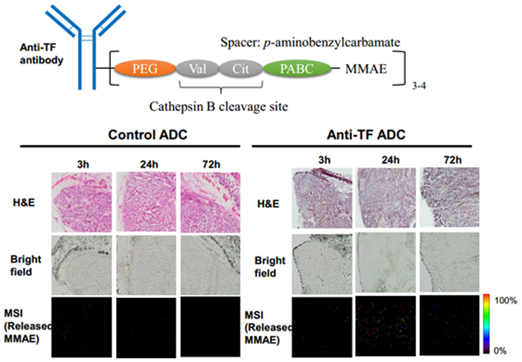
Yasunaga M, Manabe S, Tsuji A, et al. (2017) Development of antibody-drug conjugates using dds and molecular imaging. Bioengineering 4: 78. doi: 10.3390/bioengineering4030078
![]() |
[15] |
Wu C, Dill AL, Eberlin LS, et al. (2013) Mass spectrometry imaging under ambient conditions. Mass Spectrom Rev 32: 218–243. doi: 10.1002/mas.21360
![]() |
[16] |
Murray KK, Seneviratne CA, Ghorai S (2016) High resolution laser mass spectrometry bioimaging. Methods 104: 118–126. doi: 10.1016/j.ymeth.2016.03.002
![]() |
[17] |
Stoeckli M, Chaurand P, Hallahan DE, et al. (2001) Imaging mass spectrometry: A new technology for the analysis of protein expression in mammalian tissues. Nat Med 7: 493–496. doi: 10.1038/86573
![]() |
[18] |
McDonnell LA, Heeren RM (2007) Imaging mass spectrometry. Mass Spectrom Rev 26: 606–643. doi: 10.1002/mas.20124
![]() |
[19] |
Caprioli RM, Farmer TB, Gile J (1997) Molecular imaging of biological samples: Localization of peptides and proteins using maldi-tof ms. Anal Chem 69: 4751–4760. doi: 10.1021/ac970888i
![]() |
[20] |
Wulfkuhle JD, Liotta LA, Petricoin EF (2003) Proteomic applications for the early detection of cancer. Nat Rev Cancer 3: 267–275. doi: 10.1038/nrc1043
![]() |
[21] |
Fujiwara Y, Furuta M, Manabe S, et al. (2016) Imaging mass spectrometry for the precise design of antibody-drug conjugates. Sci Rep 6: 24954. doi: 10.1038/srep24954
![]() |
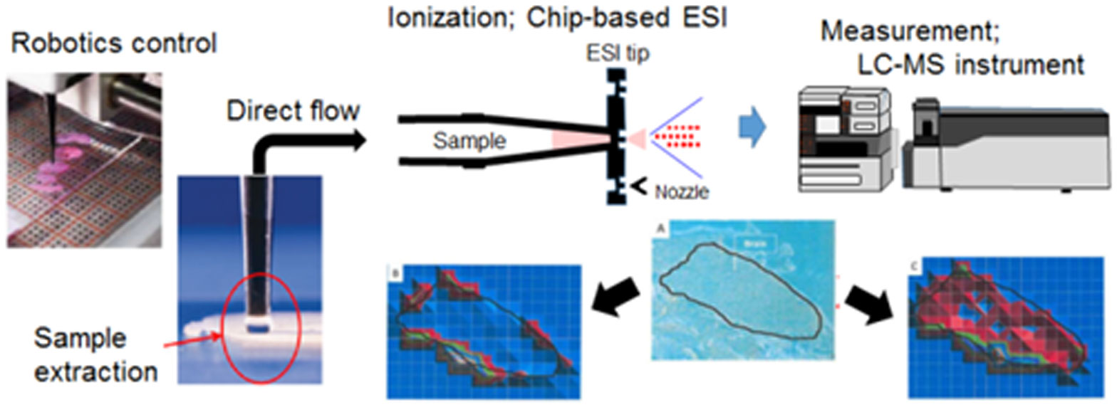
[22] | Yasunaga M, Furuta M, Ogata K, et al. (2013) The significance of microscopic mass spectrometry with high resolution in the visualisation of drug distribution. Sci Rep 3: 3050. |
[23] |
Peletier LA, Gabrielsson J (2012) Dynamics of target-mediated drug disposition: Characteristic profiles and parameter identification. J Pharmacokinet Pharmacodyn 39: 429–451. doi: 10.1007/s10928-012-9260-6
![]() |
[24] | Pineda C, Jacobs IA, Alvarez DF, et al. (2016) Assessing the immunogenicity of biopharmaceuticals. Biodrugs 30: 195–206. |
[25] |
Hampe CS (2012) Protective role of anti-idiotypic antibodies in autoimmunity-lessons for type 1 diabetes. Autoimmunity 45: 320–331. doi: 10.3109/08916934.2012.659299
![]() |
[26] |
Thomas A, Teicher BA, Hassan R (2016) Antibody-drug conjugates for cancer therapy. Lancet Oncol 17: e254–e262. doi: 10.1016/S1470-2045(16)30030-4
![]() |
[27] |
Diamantis N, Banerji U (2016) Antibody-drug conjugates-an emerging class of cancer treatment. Br J Cancer 114: 362–367. doi: 10.1038/bjc.2015.435
![]() |
[28] |
Damelin M, Zhong W, Myers J, et al. (2015) Evolving strategies for target selection for antibody-drug conjugates. Pharm Res 32: 3494–3507. doi: 10.1007/s11095-015-1624-3
![]() |
[29] |
Senter PD, Sievers EL (2012) The discovery and development of brentuximab vedotin for use in relapsed hodgkin lymphoma and systemic anaplastic large cell lymphoma. Nat Biotechnol 30: 631–637. doi: 10.1038/nbt.2289
![]() |
[30] |
Ogitani Y, Aida T, Hagihara K, et al. (2016) Ds-8201a, a novel her2-targeting adc with a novel DNA topoisomerase i inhibitor, demonstrates a promising antitumor efficacy with differentiation from t-dm1. Clin Cancer Res 22: 5097–5108. doi: 10.1158/1078-0432.CCR-15-2822
![]() |
[31] |
Sau S, Alsaab HO, Kashaw SK, et al. (2017) Advances in antibody-drug conjugates: A new era of targeted cancer therapy. Drug Discovery Today 22: 1547–1556. doi: 10.1016/j.drudis.2017.05.011
![]() |
[32] |
Mitsunaga M, Ogawa M, Kosaka N, et al. (2011) Cancer cell-selective in vivo near infrared photoimmunotherapy targeting specific membrane molecules. Nat Med 17: 1685–1691. doi: 10.1038/nm.2554
![]() |
[33] |
Larson SM, Carrasquillo JA, Cheung NK, et al. (2015) Radioimmunotherapy of human tumours. Nat Rev Cancer 15: 347–360. doi: 10.1038/nrc3925
![]() |
[34] | Sau S, Alsaab HO, Kashaw SK, et al. (2017) Advances in antibody-drug conjugates: A new era of targeted cancer therapy. Drug Discovery Today. |
[35] |
Gerber HP, Sapra P, Loganzo F, et al. (2016) Combining antibody-drug conjugates and immune-mediated cancer therapy: What to expect? Biochem Pharmacol 102: 1–6. doi: 10.1016/j.bcp.2015.12.008
![]() |
[36] |
Alsaab HO, Sau S, Alzhrani R, et al. (2017) Pd-1 and pd-l1 checkpoint signaling inhibition for cancer immunotherapy: Mechanism, combinations, and clinical outcome. Front Pharmacol 8: 561. doi: 10.3389/fphar.2017.00561
![]() |
[37] |
Matsumura Y (2014) The drug discovery by nanomedicine and its clinical experience. Jpn J Clin Oncol 44: 515–525. doi: 10.1093/jjco/hyu046
![]() |
[38] |
Nishiyama N, Matsumura Y, Kataoka K (2016) Development of polymeric micelles for targeting intractable cancers. Cancer Sci 107: 867–874. doi: 10.1111/cas.12960
![]() |
[39] | Matsumura Y, Maeda H (1986) A new concept for macromolecular therapeutics in cancer chemotherapy: Mechanism of tumoritropic accumulation of proteins and the antitumor agent smancs. Cancer Res 46: 6387–6392. |
[40] |
Cabral H, Matsumoto Y, Mizuno K, et al. (2011) Accumulation of sub-100 nm polymeric micelles in poorly permeable tumours depends on size. Nat Nanotechnol 6: 815–823. doi: 10.1038/nnano.2011.166
![]() |
[41] |
Oku N (2017) Innovations in liposomal dds technology and its application for the treatment of various diseases. Biol Pharm Bull 40: 119–127. doi: 10.1248/bpb.b16-00857
![]() |
[42] |
Kinoshita R, Ishima Y, Chuang VTG, et al. (2017) Improved anticancer effects of albumin-bound paclitaxel nanoparticle via augmentation of epr effect and albumin-protein interactions using s-nitrosated human serum albumin dimer. Biomaterials 140: 162–169. doi: 10.1016/j.biomaterials.2017.06.021
![]() |
[43] |
Duncan R (2006) Polymer conjugates as anticancer nanomedicines. Nat Rev Cancer 6: 688–701. doi: 10.1038/nrc1958
![]() |
[44] |
Yokoyama M (2014) Polymeric micelles as drug carriers: Their lights and shadows. J Drug Targeting 22: 576–583. doi: 10.3109/1061186X.2014.934688
![]() |
[45] |
Jain RK, Stylianopoulos T (2010) Delivering nanomedicine to solid tumors. Nat Rev Clin Oncol 7: 653–664. doi: 10.1038/nrclinonc.2010.139
![]() |
[46] |
Allen TM, Cullis PR (2013) Liposomal drug delivery systems: From concept to clinical applications. Adv Drug Delivery Rev 65: 36–48. doi: 10.1016/j.addr.2012.09.037
![]() |
[47] |
Bae Y, Nishiyama N, Fukushima S, et al. (2005) Preparation and biological characterization of polymeric micelle drug carriers with intracellular ph-triggered drug release property: Tumor permeability, controlled subcellular drug distribution, and enhanced in vivo antitumor efficacy. Bioconjugate Chem 16: 122–130. doi: 10.1021/bc0498166
![]() |
[48] |
Kraft JC, Freeling JP, Wang Z, et al. (2014) Emerging research and clinical development trends of liposome and lipid nanoparticle drug delivery systems. J Pharm Sci 103: 29–52. doi: 10.1002/jps.23773
![]() |
[49] | Rao W, Pan N, Yang Z (2016) Applications of the single-probe: Mass spectrometry imaging and single cell analysis under ambient conditions. J Visualized Exp JoVE 2016: 53911. |
[50] |
Calligaris D, Feldman DR, Norton I, et al. (2015) Molecular typing of meningiomas by desorption electrospray ionization mass spectrometry imaging for surgical decision-making. Int J Mass Spectrom 377: 690–698. doi: 10.1016/j.ijms.2014.06.024
![]() |
[51] |
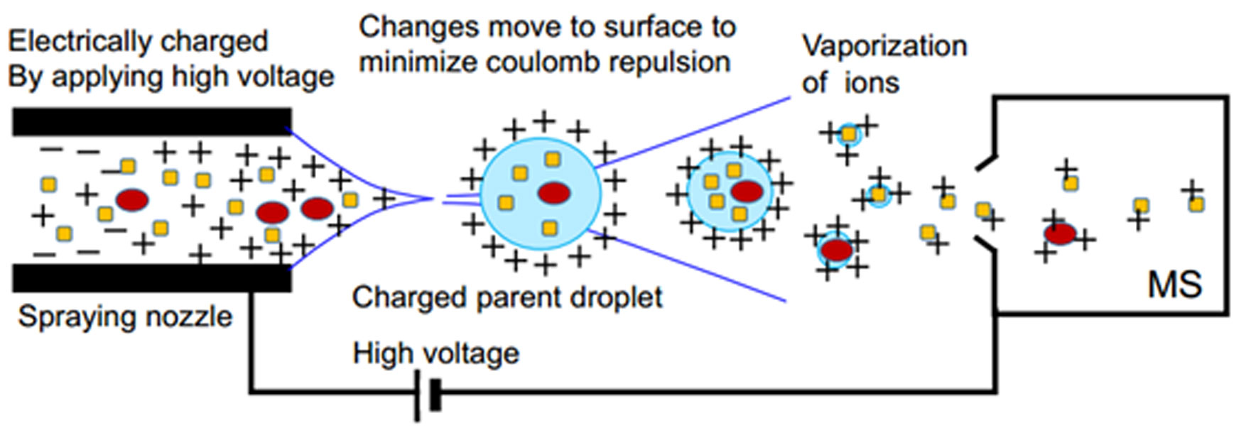
Fenn JB, Mann M, Meng CK, et al. (1989) Electrospray ionization for mass spectrometry of large biomolecules. Science 246: 64–71. doi: 10.1126/science.2675315
![]() |
[52] |
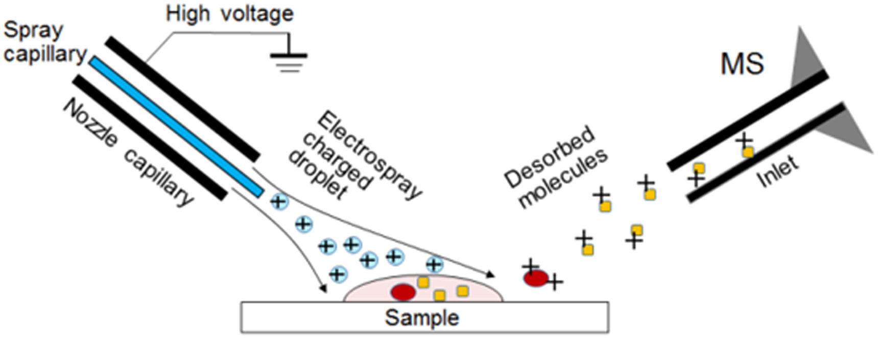
Takats Z, Wiseman JM, Gologan B, et al. (2004) Mass spectrometry sampling under ambient conditions with desorption electrospray ionization. Science 306: 471–473. doi: 10.1126/science.1104404
![]() |
[53] | Parrot D, Papazian S, Foil D, et al. (2018) Imaging the unimaginable: Desorption electrospray ionization-imaging mass spectrometry (desi-ims) in natural product research. Planta Med. |
[54] | Cooks RG, Ouyang Z, Takats Z, et al. (2006) Detection technologies. Ambient mass spectrometry. Science 311: 1566–1570. |
[55] |
Zimmerman TA, Monroe EB, Tucker KR, et al. (2008) Chapter 13: Imaging of cells and tissues with mass spectrometry: Adding chemical information to imaging. Methods Cell Biol 89: 361–390. doi: 10.1016/S0091-679X(08)00613-4
![]() |
[56] | Signor L, Boeri EE (2013) Matrix-assisted laser desorption/ionization time of flight (maldi-tof) mass spectrometric analysis of intact proteins larger than 100 kda. J Visualized Exp JoVE 108: e50635. |
[57] |
Sudhir PR, Wu HF, Zhou ZC (2005) Identification of peptides using gold nanoparticle-assisted single-drop microextraction coupled with ap-maldi mass spectrometry. Anal Chem 77: 7380–7385. doi: 10.1021/ac051162m
![]() |
[58] |
Abdelhamid HN, Wu HF (2012) A method to detect metal-drug complexes and their interactions with pathogenic bacteria via graphene nanosheet assist laser desorption/ionization mass spectrometry and biosensors. Anal Chim Acta 751: 94–104. doi: 10.1016/j.aca.2012.09.012
![]() |
[59] |
Abdelhamid HN, Wu HF (2013) Furoic and mefenamic acids as new matrices for matrix assisted laser desorption/ionization-(maldi)-mass spectrometry. Talanta 115: 442–450. doi: 10.1016/j.talanta.2013.05.050
![]() |
[60] |
Nasser AH, Wu BS, Wu HF (2014) Graphene coated silica applied for high ionization matrix assisted laser desorption/ionization mass spectrometry: A novel approach for environmental and biomolecule analysis. Talanta 126: 27–37. doi: 10.1016/j.talanta.2014.03.016
![]() |
[61] |
Abdelhamid HN, Wu HF (2015) Synthesis of a highly dispersive sinapinic acid@graphene oxide (sa@go) and its applications as a novel surface assisted laser desorption/ionization mass spectrometry for proteomics and pathogenic bacteria biosensing. Analyst 140: 1555–1565. doi: 10.1039/C4AN02158D
![]() |
[62] |
Abdelhamid HN, Wu HF (2016) Gold nanoparticles assisted laser desorption/ionization mass spectrometry and applications: From simple molecules to intact cells. Anal Bioanal Chem 408: 4485–4502. doi: 10.1007/s00216-016-9374-6
![]() |
[63] |
Harada T, Yuba-Kubo A, Sugiura Y, et al. (2009) Visualization of volatile substances in different organelles with an atmospheric-pressure mass microscope. Anal Chem 81: 9153–9157. doi: 10.1021/ac901872n
![]() |
[64] |
Saito Y, Waki M, Hameed S, et al. (2012) Development of imaging mass spectrometry. Biol Pharm Bull 35: 1417–1424. doi: 10.1248/bpb.b212007
![]() |
[65] |
Sugiura Y, Honda K, Suematsu M (2015) Development of an imaging mass spectrometry technique for visualizing localized cellular signaling mediators in tissues. Mass Spectrom 4: A0040. doi: 10.5702/massspectrometry.A0040
![]() |
[66] |
Setou M, Kurabe N (2011) Mass microscopy: High-resolution imaging mass spectrometry. J Electron Microsc 60: 47–56. doi: 10.1093/jmicro/dfq079
![]() |
[67] |
Maeda H (2001) Smancs and polymer-conjugated macromolecular drugs: Advantages in cancer chemotherapy. Adv Drug Delivery Rev 46: 169–185. doi: 10.1016/S0169-409X(00)00134-4
![]() |
[68] |
Barenholz Y (2012) Doxil(r)-the first fda-approved nano-drug: Lessons learned. J Controlled Release 160: 117–134. doi: 10.1016/j.jconrel.2012.03.020
![]() |
[69] |
Giordano G, Pancione M, Olivieri N, et al. (2017) Nano albumin bound-paclitaxel in pancreatic cancer: Current evidences and future directions. World J Gastroenterol 23: 5875–5886. doi: 10.3748/wjg.v23.i32.5875
![]() |
[70] |
Kogure K, Akita H, Yamada Y, et al. (2008) Multifunctional envelope-type nano device (mend) as a non-viral gene delivery system. Adv Drug Delivery Rev 60: 559–571. doi: 10.1016/j.addr.2007.10.007
![]() |
[71] |
Sugaya A, Hyodo I, Koga Y, et al. (2016) Utility of epirubicin-incorporating micelles tagged with anti-tissue factor antibody clone with no anticoagulant effect. Cancer Sci 107: 335–340. doi: 10.1111/cas.12863
![]() |
[72] |
Hiyama E, Ali A, Amer S, et al. (2015) Direct lipido-metabolomics of single floating cells for analysis of circulating tumor cells by live single-cell mass spectrometry. Anal Sci 31: 1215–1217. doi: 10.2116/analsci.31.1215
![]() |
[73] |
Hamaguchi T, Matsumura Y, Suzuki M, et al. (2005) Nk105, a paclitaxel-incorporating micellar nanoparticle formulation, can extend in vivo antitumour activity and reduce the neurotoxicity of paclitaxel. Br J Cancer 92: 1240–1246. doi: 10.1038/sj.bjc.6602479
![]() |
[74] |
Verma S, Miles D, Gianni L, et al. (2012) Trastuzumab emtansine for her2-positive advanced breast cancer. N Engl J Med 367: 1783–1791. doi: 10.1056/NEJMoa1209124
![]() |
[75] |
Younes A, Gopal AK, Smith SE, et al. (2012) Results of a pivotal phase ii study of brentuximab vedotin for patients with relapsed or refractory hodgkin's lymphoma. J Clin Oncol 30: 2183–2189. doi: 10.1200/JCO.2011.38.0410
![]() |
[76] |
Pro B, Advani R, Brice P, et al. (2012) Brentuximab vedotin (sgn-35) in patients with relapsed or refractory systemic anaplastic large-cell lymphoma: Results of a phase ii study. J Clin Oncol 30: 2190–2196. doi: 10.1200/JCO.2011.38.0402
![]() |
[77] |
Doronina SO, Toki BE, Torgov MY, et al. (2003) Development of potent monoclonal antibody auristatin conjugates for cancer therapy. Nat Biotechnol 21: 778–784. doi: 10.1038/nbt832
![]() |
[78] |
Lyon RP, Bovee TD, Doronina SO, et al. (2015) Reducing hydrophobicity of homogeneous antibody-drug conjugates improves pharmacokinetics and therapeutic index. Nat Biotechnol 33: 733–735. doi: 10.1038/nbt.3212
![]() |
[79] |
Hisada Y, Yasunaga M, Hanaoka S, et al. (2013) Discovery of an uncovered region in fibrin clots and its clinical significance. Sci Rep 3: 2604. doi: 10.1038/srep02604
![]() |
[80] |
Takashima H, Tsuji AB, Saga T, et al. (2017) Molecular imaging using an anti-human tissue factor monoclonal antibody in an orthotopic glioma xenograft model. Sci Rep 7: 12341. doi: 10.1038/s41598-017-12563-5
![]() |
[81] |
Koga Y, Manabe S, Aihara Y, et al. (2015) Antitumor effect of antitissue factor antibody-mmae conjugate in human pancreatic tumor xenografts. Int J Cancer 137: 1457–1466. doi: 10.1002/ijc.29492
![]() |
[82] |
Rao W, Celiz AD, Scurr DJ, et al. (2013) Ambient desi and lesa-ms analysis of proteins adsorbed to a biomaterial surface using in-situ surface tryptic digestion. J Am Soc Mass Spectrom 24: 1927–1936. doi: 10.1007/s13361-013-0737-3
![]() |
[83] | Takahashi T, Serada S, Ako M, et al. (2013) New findings of kinase switching in gastrointestinal stromal tumor under imatinib using phosphoproteomic analysis. Int J Cancer 133: 2737–2743. |
[84] |
Emara S, Amer S, Ali A, et al. (2017) Single-cell metabolomics. Adv Exp Med Biol 965: 323–343. doi: 10.1007/978-3-319-47656-8_13
![]() |
[85] |
Matsumura Y (2012) Cancer stromal targeting (cast) therapy. Adv Drug Delivery Rev 64: 710–719. doi: 10.1016/j.addr.2011.12.010
![]() |
[86] |
Yasunaga M, Manabe S, Tarin D, et al. (2011) Cancer-stroma targeting therapy by cytotoxic immunoconjugate bound to the collagen 4 network in the tumor tissue. Bioconjugate Chem 22: 1776–1783. doi: 10.1021/bc200158j
![]() |
[87] |
Yasunaga M, Manabe S, Tarin D, et al. (2013) Tailored immunoconjugate therapy depending on a quantity of tumor stroma. Cancer Sci 104: 231–237. doi: 10.1111/cas.12062
![]() |
[88] |
Yasunaga M, Manabe S, Matsumura Y (2017) Immunoregulation by il-7r-targeting antibody-drug conjugates: Overcoming steroid-resistance in cancer and autoimmune disease. Sci Rep 7: 10735. doi: 10.1038/s41598-017-11255-4
![]() |