Predator-prey dynamics with refuge, alternate food, and harvesting strategies in a patchy habitat

Rajalakshmi Manoharan; Reenu Rani; Ali Moussaoui; Rajalakshmi Manoharan; Reenu Rani; Ali Moussaoui

doi:10.3934/mbe.2025029

Mathematical Biosciences and Engineering

2025, Volume 22, Issue 4: 810-845. doi: 10.3934/mbe.2025029

Previous Article Next Article

Research article Special Issues

Predator-prey dynamics with refuge, alternate food, and harvesting strategies in a patchy habitat

1.
Department of Mathematics, School of Advanced Sciences, Vellore Institute of Technology, Vellore 632014, India
2.
Laboratory of Nonlinear Analysis and Applied Mathematics, Department of Mathematics, Faculty of Sciences, University of Tlemcen, Algeria

Received: 03 January 2025 Revised: 21 February 2025 Accepted: 28 February 2025 Published: 05 March 2025

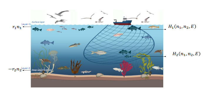
A predator–prey dynamic reaction model is investigated in a two-layered water body where only the prey is subjected to harvesting. The surface layer (Layer-1) provides food for both species, while the prey migrates to deeper layer (Layer-2) as a refuge from predation. Although the prey is the preferred food for the predator, the predator can also consume alternative food resources that are abundantly available. The availability of alternative food resources plays a crucial role in species' coexistence by mitigating the risk of extinction. The main objective of the work was to explore the effect of different harvesting strategies (nonlinear and linear harvesting) on a predator–prey model with effort dynamics in a heterogeneous habitat. The analysis incorporates a dual timescale approach: the prey species migrate between the layers on a fast timescale, whereas the growth of resource biomass, prey–predator interactions, and harvesting dynamics evolve on a slow timescale. The complete model involving both slow and fast timescales has been investigated by using aggregated model. The reduced aggregated model is analyzed analytically as well as numerically. Moreover, it is demonstrated that the reduced system exhibits the bifurcations (transcritical and Hopf point) by setting the additional food parameter as a bifurcation parameter. A comparative study using different harvesting strategies found that there is chaos in the system when using linear harvesting in the predator–prey model. However, nonlinear harvesting gives only stable or periodic solutions. This concludes that nonlinear harvesting can control the chaos in the system. Additionally, a one-dimensional parametric bifurcation, phase portraits, and time series plots are also explored in the numerical simulation.
- predator–prey model,
- effort dynamics,
- linear and nonlinear harvesting,
- alternative food,
- aggregation of variables,
- stability,
- periodic solutions,
- chaos,
- numerical simulations
Citation: Rajalakshmi Manoharan, Reenu Rani, Ali Moussaoui. Predator-prey dynamics with refuge, alternate food, and harvesting strategies in a patchy habitat[J]. Mathematical Biosciences and Engineering, 2025, 22(4): 810-845. doi: 10.3934/mbe.2025029

Related Papers:

Abstract

A predator–prey dynamic reaction model is investigated in a two-layered water body where only the prey is subjected to harvesting. The surface layer (Layer-1) provides food for both species, while the prey migrates to deeper layer (Layer-2) as a refuge from predation. Although the prey is the preferred food for the predator, the predator can also consume alternative food resources that are abundantly available. The availability of alternative food resources plays a crucial role in species' coexistence by mitigating the risk of extinction. The main objective of the work was to explore the effect of different harvesting strategies (nonlinear and linear harvesting) on a predator–prey model with effort dynamics in a heterogeneous habitat. The analysis incorporates a dual timescale approach: the prey species migrate between the layers on a fast timescale, whereas the growth of resource biomass, prey–predator interactions, and harvesting dynamics evolve on a slow timescale. The complete model involving both slow and fast timescales has been investigated by using aggregated model. The reduced aggregated model is analyzed analytically as well as numerically. Moreover, it is demonstrated that the reduced system exhibits the bifurcations (transcritical and Hopf point) by setting the additional food parameter as a bifurcation parameter. A comparative study using different harvesting strategies found that there is chaos in the system when using linear harvesting in the predator–prey model. However, nonlinear harvesting gives only stable or periodic solutions. This concludes that nonlinear harvesting can control the chaos in the system. Additionally, a one-dimensional parametric bifurcation, phase portraits, and time series plots are also explored in the numerical simulation.

References

[1]	P. K. Santra, G. S. Mahapatra, G. R. Phaijoo, Bifurcation analysis and chaos control of discrete prey–predator model incorporating novel prey–refuge concept, Comput. Math. Methods, 3 (2021), e1185. https://doi.org/10.3934/mbe.2022313 doi: 10.3934/mbe.2022313
[2]	H. Molla, Sabiar Rahman, S. Sarwardi, Dynamics of a predator–prey model with Holling type Ⅱ functional response incorporating a prey refuge depending on both the species, Int. J. Nonlinear Sci. Numer. Simul., 20 (2019), 89–104. https://doi.org/10.1515/ijnsns-2017-0224 doi: 10.1515/ijnsns-2017-0224
[3]	T. K. Kar, Stability analysis of a prey–predator model incorporating a prey refuge, Commun. Nonlinear Sci. Numer. Simul., 10 (2005), 681–691. https://doi.org/10.1016/j.cnsns.2003.08.006 doi: 10.1016/j.cnsns.2003.08.006
[4]	S. Pandey, U. Ghosh, D. Das, S. Chakraborty, A. Sarkar, Rich dynamics of a delay-induced stage-structure prey-predator model with cooperative behaviour in both species and the impact of prey refuge, Math. Comput. Simul., 216 (2024), 49–76. https://doi.org/10.1016/j.matcom.2023.09.002 doi: 10.1016/j.matcom.2023.09.002
[5]	W. Lu, Y. Xia, Y. Bai, Periodic solution of a stage-structured predator-prey model incorporating prey refuge, Math. Biosci. Eng., 17 (2020), 3160–3174. https://doi.org/10.3934/mbe.2020179 doi: 10.3934/mbe.2020179
[6]	J. Ghosh, B. Sahoo, S.Poria, Prey-predator dynamics with prey refuge providing additional food to predator, Chaos, Solitons Fractals, 96 (2017), 110–119. https://doi.org/10.1016/j.chaos.2017.01.010 doi: 10.1016/j.chaos.2017.01.010
[7]	P. D. N. Srinivasu, B. S. R. V. Prasad, M. Venkatesulu, Biological control through provision of additional food to predators: a theoretical study, Theor. Popul Biol., 72 (2007), 111–120. https://doi.org/10.1016/j.tpb.2007.03.011 doi: 10.1016/j.tpb.2007.03.011
[8]	S. Samaddar, M. Dhar, P. Bhattacharya, Effect of fear on prey–predator dynamics: Exploring the role of prey refuge and additional food, Chaos: Interdiscip. J. Nonlinear Sci., 30 (2020). https://doi.org/10.1063/5.0006968 doi: 10.1063/5.0006968
[9]	R. Rani, S. Gakkhar, The impact of provision of additional food to predator in predator–prey model with combined harvesting in the presence of toxicity, J. Appl. Math. Comput., 60 (2019), 673–701. https://doi.org/10.1007/s12190-018-01232-z doi: 10.1007/s12190-018-01232-z
[10]	D. K. Jana, P. Panja, Effects of supplying additional food for a scavenger species in a prey-predator-scavenger model with quadratic harvesting, Int. J. Modell. Simul., 43 (2022), 250–264. https://doi.org/10.1080/02286203.2022.2065658 doi: 10.1080/02286203.2022.2065658
[11]	P. Panja, S. Jana, S. Kumar Mondal, Effects of additional food on the dynamics of a three species food chain model incorporating refuge and harvesting, Int. J. Nonlinear Sci. Numer. Simul., 20 (2019), 787–801. https://doi.org/10.1515/ijnsns-2018-0313 doi: 10.1515/ijnsns-2018-0313
[12]	M. Kaur, R. Rani, R. Bhatia, G. N. Verma, S. Ahiwar, Dynamical study of quadrating harvesting of a predator–prey model with Monod–Haldane functional response, J. Appl. Math. Comput., 66 (2021), 397–422. https://doi.org/10.1007/s12190-020-01438-0 doi: 10.1007/s12190-020-01438-0
[13]	S. R. Jawad, M. Al Nuaimi, Persistence and bifurcation analysis among four species interactions with the influence of competition, predation and harvesting, Iraqi J. Sci., (2023), 1369–1390. https://doi.org/10.24996/ijs.2023.64.3.30 doi: 10.24996/ijs.2023.64.3.30
[14]	S. Tolcha, B. K. Bole, P. R. Koya, Population dynamics of two mutuality preys and one predator with harvesting of one prey and allowing alternative food source to predator, Math. Model. Appl., 5 (2020), 55. https://doi.org/10.11648/j.mma.20200502.12 doi: 10.11648/j.mma.20200502.12
[15]	D. S. Al-Jaf, The role of linear type of harvesting on two competitive species interaction, Commun. Math. Biol. Neurosci., (2024). lhttps://doi.org/10.28919/cmbn/8426
[16]	Y. Wang, X. Zhou, W. Jiang, Bifurcations in a diffusive predator-prey system with linear harvesting, Chaos, Solitons Fractals, 169 (2023), 113286. https://doi.org/10.1016/j.chaos.2023.113286 doi: 10.1016/j.chaos.2023.113286
[17]	M. Chen, W. Yang, Effect of non-linear harvesting and delay on a predator-prey model with Beddington-DeAngelis functional response, Commun. Math. Biol. Neurosci., 2024. https://doi.org/10.28919/cmbn/8382
[18]	S. Pal, S. Majhi, S. Mandal, N. Pal, Role of fear in a predator-prey model with Beddington–DeAngelis functional response, Z. Naturforsch. A, 74 (2019), 581–595. https://doi.org/10.1515/zna-2018-0449 doi: 10.1515/zna-2018-0449
[19]	R. Rani, S. Gakkhar, A. Moussaoui, Dynamics of a fishery system in a patchy environment with nonlinear harvesting, Math. Methods Appl. Sci., 42 (2019), 7192–7209. https://doi.org/10.1002/mma.5826 doi: 10.1002/mma.5826
[20]	R. Rani, S. Gakkhar, Non-linear effort dynamics for harvesting in a Predator- Prey system, J. Nat. Sci. Res., 5 (2015).
[21]	M. Li, B. Chen, H. Ye, A bioeconomic differential algebraic predator–prey model with nonlinear prey harvesting, Appl. Math. Modell., 42 (2017), 17–28. https://doi.org/10.1016/j.apm.2016.09.029 doi: 10.1016/j.apm.2016.09.029
[22]	J. C. Poggiale, P. Auger, Impact of spatial heterogeneity on a predator–prey system dynamics, C.R. Biol., 327 (2004), 1058–1063. https://doi.org/10.1016/j.crvi.2004.06.006 doi: 10.1016/j.crvi.2004.06.006
[23]	S. A. Levin, Population dynamic models in heterogeneous environments, Ann. Rev. Ecol. Syst., 7 (1976), 287–310.
[24]	K. Dao Duc, P. Augera, T. Nguyen-Huu, Predator density-dependent prey dispersal in a patchy environment with a refuge for the prey: biological modelling, S. Afr. J. Sci., 104 (2008), 180–184.
[25]	R. Mchich, P. Auger, J. C. Poggiale, Effect of predator density dependent dispersal of prey on stability of a predator-prey system, Math. Biosci., 206 (2007), 343–356. https://doi.org/10.1016/j.mbs.2005.11.005 doi: 10.1016/j.mbs.2005.11.005
[26]	A. El Abdllaoui, P. Auger, B.W. Kooi, R. B. De la Parra, R. Mchich, Effects of density-dependent migrations on stability of a two-patch predator–prey model, Math. Biosci., 210 (2007), 335–354. https://doi.org/10.1016/j.mbs.2007.03.002 doi: 10.1016/j.mbs.2007.03.002
[27]	A. Moussaoui, P. Auger, Simple fishery and marine reserve models to study the SLOSS problem, ESAIM: Proc. Surv., 49 (2015), 78–90. https://doi.org/10.1051/proc/201549007 doi: 10.1051/proc/201549007
[28]	M. Bensenane, A. Moussaoui, P. Auger, On the optimal size of marine reserves, Acta Biotheor., 61 (2013), 109–118. https://doi.org/10.1007/s10441-013-9173-9 doi: 10.1007/s10441-013-9173-9
[29]	A. Moussaoui, M. Bensenane, P. Auger, A. Bah, On the optimal size and number of reserves in a multi-site fishery model, J. Biol. Syst., 22 (2014), 1–17.
[30]	J. Carr, Applications of Centre Manifold Theory, Springer, 1981. https://doi.org/10.1007/978-1-4612-5929-9
[31]	P. Auger, R. B. De la Parra, J. C. Poggiale, E. Sánchez, T. Nguyen-Huu, Aggregation of variables and applications to population dynamics, Struct. Popul. Models Biol. Epidemiol., (2008), 209–263. https://doi.org/10.1007/978-3-540-78273-55
[32]	T. Grozdanovski, J. J. Shepherd, A. Stacey, Multi-scaling analysis of a logistic model with slowly varying coefficients, Appl. Math. Lett., 22 (2009), 1091–1095. https://doi.org/10.1016/j.aml.2008.10.002 doi: 10.1016/j.aml.2008.10.002
[33]	M. H. Holmes, Introduction to Perturbation Methods, Springer, 1995. https://doi.org/10.1002/zamm.19960760709
[34]	P. Auger, S. Charles, M. Viala, J. C. Poggiale, Aggregation and emergence in ecological modelling: integration of ecological levels, Ecol. Modell., 127 (2000), 11–20. https://doi.org/10.1016/S0304-3800(99)00201-X doi: 10.1016/S0304-3800(99)00201-X
[35]	W. M. Liu, Criterion of Hopf bifurcations without using eigenvalues, J. Math. Anal. Appl., 182 (1994), 250–256. https://doi.org/10.1006/jmaa.1994.1079 doi: 10.1006/jmaa.1994.1079
[36]	D. Sen, S. Ghorai, M. Banerjee, Complex dynamics of a three species prey-predator model with intraguild predation, Ecol. Complexity, 34 (2018), 9–22. https://doi.org/10.1016/j.ecocom.2018.02.002 doi: 10.1016/j.ecocom.2018.02.002
[37]	R. P. Gupta, M. Banerjee, P. Chandra, Period doubling cascades of prey-predator model with nonlinear harvesting and control of over exploitation through taxation, Commun. Nonlinear Sci. Numer. Simul., 19 (2014), 2382–2405. https://doi.org/10.1016/j.cnsns.2013.10.033 doi: 10.1016/j.cnsns.2013.10.033
[38]	W. Govaerts, Y. A. Kuznetsov, A. Dhooge, Numerical continuation of bifurcations of limit cycles in MATLAB, SIAM J. Sci. Comput., 27 (2005), 231–252. https://doi.org/10.1137/030600746 doi: 10.1137/030600746
[39]	A. Riet, A Continuation Toolbox in Matlab, Master's thesis, Mathematical Institute, Utrecht University, Utrecht, The Netherlands, 2000.
[40]	W. Mestrom, Continuation of Limit Cycles in MATLAB, Master's thesis, Mathematical Institute, Utrecht University, Utrecht, The Netherlands, 2002.
[41]	A. Dhooge, W. Govaerts, Y. A. Kuznetsov, MATCONT: A MATLAB package for numerical bifurcation analysis of ODEs, ACM Trans. Math. Software (TOMS), 90 (2003), 141–164. https://doi.org/10.1145/779359.779362 doi: 10.1145/779359.779362

Reader Comments

Your name:*

Email:*
© 2025 the Author(s), licensee AIMS Press. This is an open access article distributed under the terms of the Creative Commons Attribution License (http://creativecommons.org/licenses/by/4.0)