Modeling localized corrosion in biofuel storage tanks

Hossein Moradi; Gabriele Grifò; Maria Francesca Milazzo; Edoardo Proverbio; Giancarlo Consolo; Hossein Moradi; Gabriele Grifò; Maria Francesca Milazzo; Edoardo Proverbio; Giancarlo Consolo

doi:10.3934/mbe.2025025

Mathematical Biosciences and Engineering

2025, Volume 22, Issue 3: 677-699. doi: 10.3934/mbe.2025025

Previous Article Next Article

Research article Special Issues

Modeling localized corrosion in biofuel storage tanks

1.
Department of Mathematical, Computer, Physical and Earth Sciences, University of Messina, V.le F. Stagno D'Alcontres, 31 Messina, 98166, Italy
2.
Department of Engineering, University of Messina, C.da Di Dio, s/n, Messina, 98166, Italy

Academic Editor: Mingji Zhang

Received: 08 November 2024 Revised: 23 January 2025 Accepted: 10 February 2025 Published: 27 February 2025

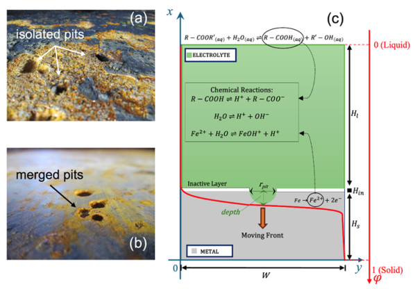
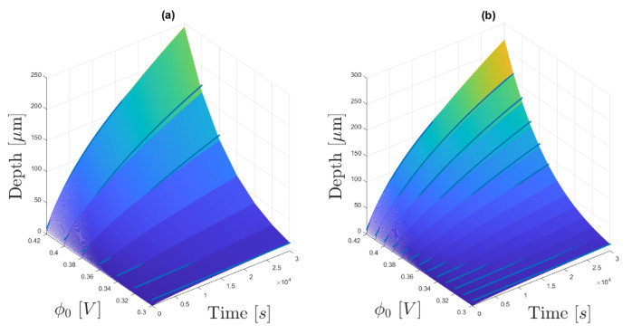
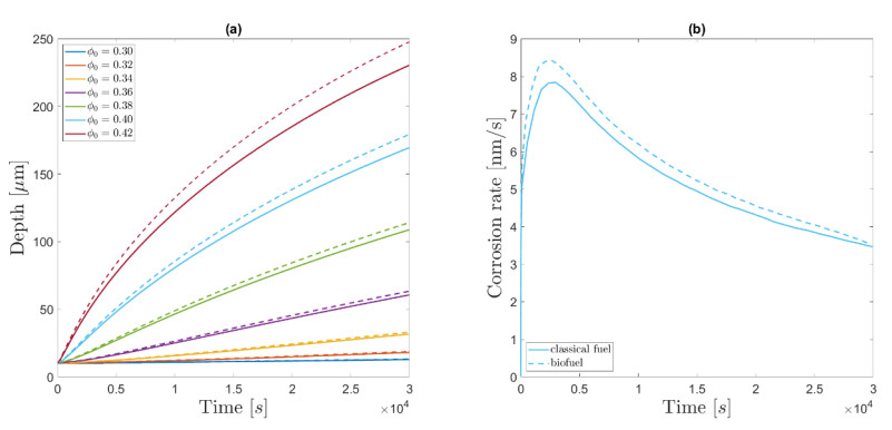
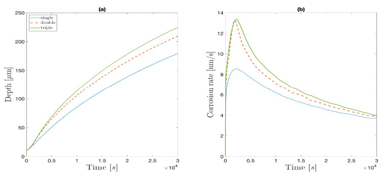
This work aims to model the influence of biofuels on localized "pitting" corrosion that occurs at the bottom of atmospheric storage tanks. To achieve this purpose, an electro-chemical phase-field model is proposed to include the extra chemical reaction due to the presence of organic acids in an electrolyte solution. The resulting set of nonlinear coupled partial differential equations is numerically integrated by means of finite element methods with a twofold aim: tracking the evolution of the metal/electrolyte interface and predicting the corrosion rates observed when either single or multiple interacting pits are formed in the bottom of a carbon steel tank. The results obtained in the case of single pit, which exhibited a good quantitative agreement with recent experimental data, can be summarized as follows: the presence of organic acids led to higher corrosion rates in comparison with conventional fuels; the corrosion rate is a two-stage process; the dependence of the pit depth as a function of time; and the solid potential, which can be successfully described via a double power law. For multiple interacting pits, the larger corrosivity associated to biofuels was further amplified and the long-time behavior of pit growth gave rise to a "band" behavior, with the major role being played by the number of pits rather than the initial spacings among them. Thus, the proposed model can be employed as a sophisticated tool to predict and quantify the real hazards associated with the release of pollutants in the environment, as well as to optimize the maintenance strategies based on an improved risk-based inspection planning.
- pitting corrosion,
- computational modeling,
- biofuels,
- electro-chemo phase-field models,
- partial differential equations
Citation: Hossein Moradi, Gabriele Grifò, Maria Francesca Milazzo, Edoardo Proverbio, Giancarlo Consolo. Modeling localized corrosion in biofuel storage tanks[J]. Mathematical Biosciences and Engineering, 2025, 22(3): 677-699. doi: 10.3934/mbe.2025025

Related Papers:

Abstract

This work aims to model the influence of biofuels on localized "pitting" corrosion that occurs at the bottom of atmospheric storage tanks. To achieve this purpose, an electro-chemical phase-field model is proposed to include the extra chemical reaction due to the presence of organic acids in an electrolyte solution. The resulting set of nonlinear coupled partial differential equations is numerically integrated by means of finite element methods with a twofold aim: tracking the evolution of the metal/electrolyte interface and predicting the corrosion rates observed when either single or multiple interacting pits are formed in the bottom of a carbon steel tank. The results obtained in the case of single pit, which exhibited a good quantitative agreement with recent experimental data, can be summarized as follows: the presence of organic acids led to higher corrosion rates in comparison with conventional fuels; the corrosion rate is a two-stage process; the dependence of the pit depth as a function of time; and the solid potential, which can be successfully described via a double power law. For multiple interacting pits, the larger corrosivity associated to biofuels was further amplified and the long-time behavior of pit growth gave rise to a "band" behavior, with the major role being played by the number of pits rather than the initial spacings among them. Thus, the proposed model can be employed as a sophisticated tool to predict and quantify the real hazards associated with the release of pollutants in the environment, as well as to optimize the maintenance strategies based on an improved risk-based inspection planning.

References

[1]	L. Cherwoo, I. Gupta, G. Flora, R. Verma, M. Kapil, S. K. Arya, et al., Biofuels an alternative to traditional fossil fuels: A comprehensive review, Sustain. Energ. Technol. Assess. , 60 (2023), 103503. https://doi.org/10.1016/j.seta.2023.103503 doi: 10.1016/j.seta.2023.103503
[2]	M. V. Rodionova, R. S. Poudyal, I. Tiwari, R. A. Voloshin, S. K. Zharmukhamedov, H. G. Nam, et al., Biofuel production: Challenges and opportunities, Int. J. Hydrogen Energ. , 42 (2017), 8450–8461. https://doi.org/10.1016/j.ijhydene.2016.11.125 doi: 10.1016/j.ijhydene.2016.11.125
[3]	API Standard 650, 13th Ed., Available from: https://www.api.org/products-and-services/standards/important-standards-announcements/standard650.
[4]	N. Perez, Electrochemical corrosion, in Electrochemistry and Corrosion Science, Springer International Publishing, Cham, (2016), 1–23. https://doi.org/10.1007/978-3-319-24847-9_1
[5]	D. A. Shifler, Localized corrosion, in Corrosion in Marine Environments, John Wiley & Sons, Inc., (2022), 63–121. https://doi.org/10.1002/9781119788867.ch4
[6]	J. R. Galvele, Pitting corrosion, in Treatise on Materials Science and Technology (ed. J. C. Scully), Elsevier, (1983), 1–57. https://doi.org/10.1016/B978-0-12-633670-2.50006-1
[7]	L. N. Komariah, S. Arita, B. E. Prianda, T. K. Dewi, Technical assessment of biodiesel storage tank: a corrosion case study, J. King Saud. Univ. Eng. Sci., 35 (2023), 232–237. https://doi.org/10.1016/j.jksues.2021.03.016 doi: 10.1016/j.jksues.2021.03.016
[8]	M. F. Milazzo, G. Ancione, P. Bragatto, E. Proverbio, A probabilistic approach for the estimation of the residual useful lifetime of atmospheric storage tanks in oil industry, J. Loss Prevent. Proc. Ind. , 77 (2022), 104781. https://doi.org/10.1016/j.jlp.2022.104781 doi: 10.1016/j.jlp.2022.104781
[9]	C. A. Shargay, K. Moore, M. West, NACE-2014-3729, Corrosion 2014, San Antonio, Texas, USA, 2014.
[10]	K. A. Zahan, M. Kano, Biodiesel production from palm oil, its by-products, and mill effluent: A review, Energies, 11 (2018), 2132. https://doi.org/10.3390/en11082132 doi: 10.3390/en11082132
[11]	M. Rostami, S. Raeissi, M. Mahmoodi, M. Nowroozi, Liquid–Liquid equilibria in biodiesel production, J. Am. Oil Chem. Soc. , 90 (2013), 147–154. https://doi.org/10.1007/s11746-012-2144-5 doi: 10.1007/s11746-012-2144-5
[12]	A. Groysman, Corrosion in Systems for Storage and Transportation of Petroleum Products and Biofuels: Identification, Monitoring and Solutions, Springer Dordrecht, 2014. https://doi.org/10.1007/978-94-007-7884-9
[13]	H. Parangusan, J. Bhadra, N. Al-Thani, A review of passivity breakdown on metal surfaces: influence of chloride- and sulfide-ion concentrations, temperature, and pH, Emerg. Mater. , 4 (2021), 1187–1203. https://doi.org/10.1007/s42247-021-00194-6 doi: 10.1007/s42247-021-00194-6
[14]	Y. Tan, Understanding the effects of electrode inhomogeneity and electrochemical heterogeneity on pitting corrosion initiation on bare electrode surfaces, Corros. Sci. , 53 (2011), 1845–1864. https://doi.org/10.1016/j.corsci.2011.02.002 doi: 10.1016/j.corsci.2011.02.002
[15]	EEMUA Publication 159 Digital, Available from: https://www.eemua.org/Products/Publications/Digital/EEMUA-Publication-159.aspx.
[16]	API 580 - Risk Based Inspection, 2023. Available from: https://www.api.org/products-and-services/individual-certification-programs/certifications/api580.
[17]	C. Cui, R. Ma, E. Martínez-Pañeda, Electro-chemo-mechanical phase field modeling of localized corrosion: theory and COMSOL implementation, Eng. Comput. , 39 (2023), 3877–3894. https://doi.org/10.1007/s00366-023-01833-8 doi: 10.1007/s00366-023-01833-8
[18]	W. J. Boettinger, J. A. Warren, C. Beckermann, A. Karma, Phase-field simulation of solidification, Annu. Rev. Mater. Res. , 32 (2002), 163–194. https://doi.org/10.1146/annurev.matsci.32.101901.155803 doi: 10.1146/annurev.matsci.32.101901.155803
[19]	W. Mai, S. Soghrati, R. G. Buchheit, A phase field model for simulating the pitting corrosion, Corros. Sci. , 110 (2016), 157–166. https://doi.org/10.1016/j.corsci.2016.04.001 doi: 10.1016/j.corsci.2016.04.001
[20]	C. Cui, R. Ma, E. Martínez-Pañeda, A phase field formulation for dissolution-driven stress corrosion cracking, J. Mech. Phys. Solids, 147 (2021), 104254. https://doi.org/10.1016/j.jmps.2020.104254 doi: 10.1016/j.jmps.2020.104254
[21]	S. M. Sharland, P. W. Tasker, A mathematical model of crevice and pitting corrosion—Ⅰ. The physical model, Corros. Sci. , 28 (1988), 603–620. https://doi.org/10.1016/0010-938X(88)90027-3 doi: 10.1016/0010-938X(88)90027-3
[22]	A. T. Hoang, M. Tabatabaei, M. Aghbashlo, A review of the effect of biodiesel on the corrosion behavior of metals/alloys in diesel engines, Energy Sources Part A, 42 (2020), 2923–2943. https://doi.org/10.1080/15567036.2019.1623346 doi: 10.1080/15567036.2019.1623346
[23]	J. W. Cahn, J. E. Hilliard, Free energy of a nonuniform system. Ⅰ. interfacial free energy, J. Chem. Phys. , 28 (1958), 258–267. https://doi.org/10.1063/1.1744102 doi: 10.1063/1.1744102
[24]	S. M. Sharland, A mathematical model of crevice and pitting corrosion—Ⅱ. The mathematical solution, Corros. Sci. , 28 (1988), 621–630. https://doi.org/10.1016/0010-938X(88)90028-5 doi: 10.1016/0010-938X(88)90028-5
[25]	S. G. Kim, W. T. Kim, T. Suzuki, Phase-field model for binary alloys, Phys. Rev. E, 60 (1999), 7186–7197. https://doi.org/10.1103/PhysRevE.60.7186 doi: 10.1103/PhysRevE.60.7186
[26]	S. M. Sharland, C. P. Jackson, A. J. Diver, A finite-element model of the propagation of corrosion crevices and pits, Corros. Sci. , 29 (1989), 1149–1166. https://doi.org/10.1016/0010-938X(89)90051-6 doi: 10.1016/0010-938X(89)90051-6
[27]	L. M. Baena, J. A. Calderón, Effects of palm biodiesel and blends of biodiesel with organic acids on metals, Heliyon, 6 (2020), e03735. https://doi.org/10.1016/j.heliyon.2020.e03735 doi: 10.1016/j.heliyon.2020.e03735
[28]	B. E. McNealy, J. L. Hertz, Extended Poisson–Nernst–Planck modeling of membrane blockage via insoluble reaction products, J. Math. Chem. , 52 (2014), 430–440. https://doi.org/10.1007/s10910-013-0270-4 doi: 10.1007/s10910-013-0270-4
[29]	COMSOL Multiphysics® v. 6.2 (2023), COMSOL AB, Stockholm, Sweden. Available from: http://www.comsol.com.
[30]	J. Bhandari, F. Khan, R. Abbassi, V. Garaniya, R. Ojeda, Modelling of pitting corrosion in marine and offshore steel structures – A technical review, J. Loss Prevent. Proc. Ind. , 37 (2015), 39–62. https://doi.org/10.1016/j.jlp.2015.06.008 doi: 10.1016/j.jlp.2015.06.008
[31]	M. A. Reinsel, J. J. Borkowski, J. T. Sears, Partition coefficients for acetic, propionic, and butyric acids in a crude oil/water system, J. Chem. Eng. Data, 39 (1994), 513–516. https://doi.org/10.1021/je00015a026 doi: 10.1021/je00015a026
[32]	J. E. McMurry, R. C. Fay, Chemistry, 6th ed., Pearson Education, 2011.
[33]	J. Drzymala, Chemical equilibria in the oleic acid-water-NaCl system, J. Colloid Interface Sci. , 108 (1985), 257–263. https://doi.org/10.1016/0021-9797(85)90259-0 doi: 10.1016/0021-9797(85)90259-0
[34]	P. Atkins, J. de Paula, R. Friedman, Physical Chemistry: Quanta, Matter, and Change, OUP Oxford, 2014. https://doi.org/10.1093/hesc/9780199609819.001.0001
[35]	B. Rangarajan, A. Havey, E. A. Grulke, P. D. Culnan, Kinetic parameters of a two-phase model for in situ epoxidation of soybean oil, J. Am. Oil Chem. Soc. , 72 (1995), 1161–1169. https://doi.org/10.1007/BF02540983 doi: 10.1007/BF02540983
[36]	D. Gamaralalage, O. Sawai, T. Nunoura, Degradation behavior of palm oil mill effluent in Fenton oxidation, J. Hazard. Mater., 364 (2019), 791–799. https://doi.org/10.1016/j.jhazmat.2018.07.023 doi: 10.1016/j.jhazmat.2018.07.023
[37]	National Center for Biotechnology Information, PubChem Compound Summary for CID 985, Palmitic Acid, 2025. Available from: https://pubchem.ncbi.nlm.nih.gov/compound/Palmitic-Acid.
[38]	Y. Katano, K. Miyata, H. Shimizu, T. Isogai, Predictive model for pit growth on underground pipes, Corrosion, 59 (2003), 155–161. https://doi.org/10.5006/1.3277545 doi: 10.5006/1.3277545
[39]	F. Pessu, R. Barker, A. Neville, Understanding pitting corrosion behavior of X65 carbon steel in CO₂-saturated environments: The temperature effect, Corrosion, 72 (2015), 78–94. https://doi.org/10.5006/1338 doi: 10.5006/1338
[40]	F. Pessu, R. Barker, A. Neville, CO₂ corrosion of carbon steel: The synergy of chloride ion concentration and temperature on metal penetration, Corrosion, 76 (2020), 957–974. https://doi.org/10.5006/3583 doi: 10.5006/3583
[41]	M. A. Fazal, A. S. M. A. Haseeb, H. H. Masjuki, Corrosion mechanism of copper in palm biodiesel, Corros. Sci. , 67 (2013), 50–59. https://doi.org/10.1016/j.corsci.2012.10.006 doi: 10.1016/j.corsci.2012.10.006
[42]	M. Ghahari, D. Krouse, N. Laycock, T. Rayment, C. Padovani, M. Stampanoni, et al., Synchrotron X-ray radiography studies of pitting corrosion of stainless steel: Extraction of pit propagation parameters, Corros. Sci. , 100 (2015), 23–35. https://doi.org/10.1016/j.corsci.2015.06.023 doi: 10.1016/j.corsci.2015.06.023
[43]	T. Q. Ansari, Z. Xiao, S. Hu, Y. Li, J. L. Luo, S. Q. Shi, Phase-field model of pitting corrosion kinetics in metallic materials, NPJ Comput. Mater. , 4 (2018), 38. https://doi.org/10.1038/s41524-018-0089-4 doi: 10.1038/s41524-018-0089-4

Reader Comments

Your name:*

Email:*
© 2025 the Author(s), licensee AIMS Press. This is an open access article distributed under the terms of the Creative Commons Attribution License (http://creativecommons.org/licenses/by/4.0)