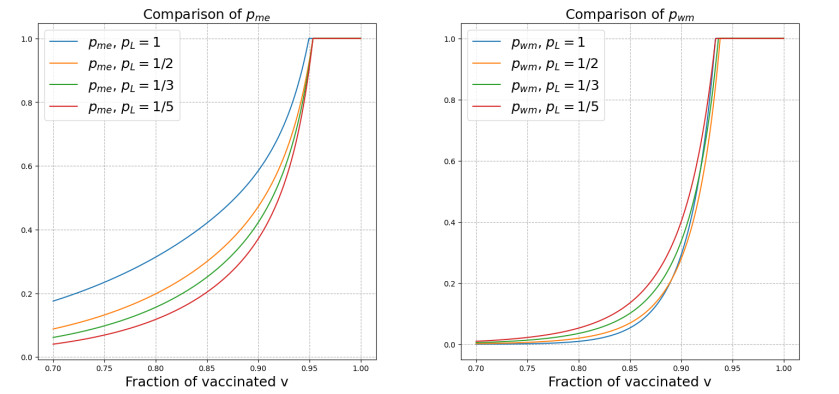
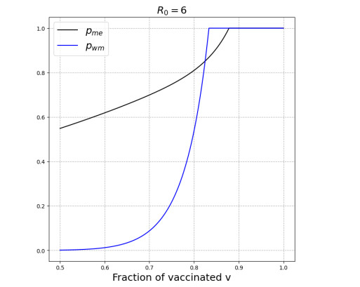
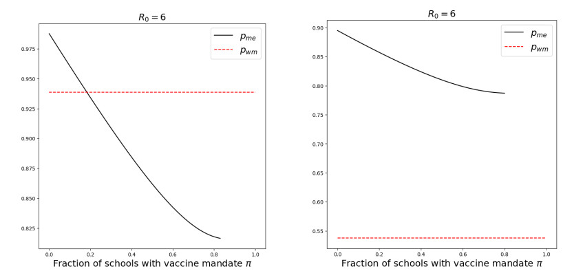
We modeled the impact of local vaccine mandates on the spread of vaccine-preventable infectious diseases, which in the absence of vaccines will mainly affect children. Examples of such diseases are measles, rubella, mumps, and pertussis. To model the spread of the pathogen, we used a stochastic SIR (susceptible, infectious, recovered) model with two levels of mixing in a closed population, often referred to as the household model. In this model, individuals make local contacts within a specific small subgroup of the population (e.g., within a household or a school class), while they also make global contacts with random people in the population at a much lower rate than the rate of local contacts. We considered what would happen if schools were given freedom to impose vaccine mandates on all of their pupils, except for the pupils that were exempt from vaccination because of medical reasons. We investigated first how such a mandate affected the probability of an outbreak of a disease. Furthermore, we focused on the probability that a pupil that was medically exempt from vaccination, would get infected during an outbreak. We showed that if the population vaccine coverage was close to the herd-immunity level, then both probabilities may increase if local vaccine mandates were implemented. This was caused by unvaccinated pupils possibly being moved to schools without mandates.
Citation: Maddalena Donà, Pieter Trapman. Possible counter-intuitive impact of local vaccine mandates for vaccine-preventable infectious diseases[J]. Mathematical Biosciences and Engineering, 2024, 21(7): 6521-6538. doi: 10.3934/mbe.2024284
We modeled the impact of local vaccine mandates on the spread of vaccine-preventable infectious diseases, which in the absence of vaccines will mainly affect children. Examples of such diseases are measles, rubella, mumps, and pertussis. To model the spread of the pathogen, we used a stochastic SIR (susceptible, infectious, recovered) model with two levels of mixing in a closed population, often referred to as the household model. In this model, individuals make local contacts within a specific small subgroup of the population (e.g., within a household or a school class), while they also make global contacts with random people in the population at a much lower rate than the rate of local contacts. We considered what would happen if schools were given freedom to impose vaccine mandates on all of their pupils, except for the pupils that were exempt from vaccination because of medical reasons. We investigated first how such a mandate affected the probability of an outbreak of a disease. Furthermore, we focused on the probability that a pupil that was medically exempt from vaccination, would get infected during an outbreak. We showed that if the population vaccine coverage was close to the herd-immunity level, then both probabilities may increase if local vaccine mandates were implemented. This was caused by unvaccinated pupils possibly being moved to schools without mandates.

| [1] | World Health Organisation, Measles, 2023. Available from: https://www.who.int/news-room/fact-sheets/detail/measles. |
| [2] |
S. Thompson, J. C. Meyer, R. J. Burnett, S. M. Campbell, Mitigating vaccine hesitancy and building trust to prevent future measles outbreaks in England, Vaccines, 11 (2023), 288. https://doi.org/10.3390/vaccines11020288 doi: 10.3390/vaccines11020288

|
| [3] | O. Diekmann, H. Heesterbeek, T. Britton, Mathematical Tools for Understanding Infectious Disease Dynamics, Princeton University Press, 2013. |
| [4] | World Health Organisation, History of Measles Vaccine, Available from: https://www.who.int/news-room/spotlight/history-of-vaccination/history-of-measles-vaccination. |
| [5] | Ministero della Salute (Italian Ministery of Health), Legge Vaccini, 2024. Available from: https://www.salute.gov.it/portale/vaccinazioni/dettaglioContenutiVaccinazioni.jsp?id = 4824 & area = vaccinazioni & menu = vuoto. |
| [6] | Eerste Kamer (Dutch Senate), Initiatiefvoorstel-Raemakers en Van Meenen, 2022. Available from: https://www.eerstekamer.nl/wetsvoorstel/35049_initiatiefvoorstel_raemakers. |
| [7] |
K. Wiley, M. Christou-Ergos, C. Degeling, R. McDougall, P. Robinson, K. Attwell, et al., Childhood vaccine refusal and what to do about it: a systematic review of the ethical literature, BMC Med. Ethics, 24 (2023), 96. https://doi.org/10.1186/s12910-023-00978-x doi: 10.1186/s12910-023-00978-x
|
| [8] | World Health Organisation, Ten Threats to Global Health in 2019. Available from: https://www.who.int/news-room/spotlight/ten-threats-to-global-health-in-2019. |
| [9] | World Health Organisation, Infodemics and Misinformation Negatively Affect People's Health Behaviours, New Who Review Finds, 2022. Available from: https://www.who.int/europe/news/item/01-09-2022-infodemics-and-misinformation-negatively-affect-people-s-health-behaviours–new-who-review-finds. |
| [10] |
W. L. M. Ruijs, J. L. A. Hautvast, G. van IJzendoorn, W. J. C. van Ansem, K. van der Velden, M. E. Hulscher, How orthodox protestant parents decide on the vaccination of their children: a qualitative study, BMC Public Health, 12 (2012), 408. https://doi.org/10.1186/1471-2458-12-408 doi: 10.1186/1471-2458-12-408
|
| [11] | H. Andersson, T. Britton, Stochastic Epidemic Models and Their Statistical Analysis, Springer Science & Business Media, 2000. |
| [12] |
K. Kuulasmaa, The spatial general epidemic and locally dependent random graphs, J. Appl. Probab., 19 (1982), 745–758. https://doi.org/10.2307/3213827 doi: 10.2307/3213827
|
| [13] |
J. Hübschen, I. Gouandjika-Vasilache, J. Dina, Measles, Lancet, 399 (2022), 678–690. https://doi.org/10.1016/S0140-6736(21)02004-3 doi: 10.1016/S0140-6736(21)02004-3
|
| [14] |
F. Ball, D. Mollison, G. Scalia-Tomba, Epidemics with two levels of mixing, Ann. Appl. Probab., 7 (1997), 46–89. https://doi.org/10.1214/aoap/1034625252 doi: 10.1214/aoap/1034625252
|
| [15] |
L. Pellis, F. Ball, P. Trapman, Reproduction numbers for epidemic models with households and other social structures, Ⅰ. definition and calculation of ${R}_0$, Math. Biosci., 235 (2012), 85–97. https://doi.org/10.1016/j.mbs.2011.10.009 doi: 10.1016/j.mbs.2011.10.009
|
| [16] |
F. Ball, L. Pellis, P. Trapman, Reproduction numbers for epidemic models with households and other social structures Ⅱ: Comparisons and implications for vaccination, Math. Biosci., 274 (2013), 108–139. https://doi.org/10.1016/j.mbs.2016.01.006 doi: 10.1016/j.mbs.2016.01.006
|
| [17] |
N. G. Becker, K. Dietz, The effect of household distribution on transmission and control of highly infectious diseases, Math. Biosci., 127 (1995), 207–219. https://doi.org/10.1016/0025-5564(94)00055-5 doi: 10.1016/0025-5564(94)00055-5
|
| [18] |
T. Britton, K. Y. Leung, P. Trapman, Who is the infector? general multi-type epidemics and real-time susceptibility processes, Adv. Appl. Probab., 51 (2019), 606–631. https://doi.org/10.1017/apr.2019.25 doi: 10.1017/apr.2019.25
|
| [19] | P. Jagers, Branching Processes with Biological Applications, Wiley, 1975. |
| [20] |
F. Ball, O. D. Lyne, Stochastic multi-type SIR epidemics among a population partitioned into households, Adv. Appl. Probab., 33 (2001), 99–123. https://doi.org/10.1017/S000186780001065X doi: 10.1017/S000186780001065X
|
| [21] | G. Grimmett, D. Stirzaker, Probability and Random Processes, 3rd edition, Oxford University Press, 2002. |
Figures(11)

Maddalena Donà, Pieter Trapman. Possible counter-intuitive impact of local vaccine mandates for vaccine-preventable infectious diseases[J]. Mathematical Biosciences and Engineering, 2024, 21(7): 6521-6538. doi: 10.3934/mbe.2024284


 DownLoad: