Modeling and analyzing an opinion network dynamics considering the environmental factor

Fulian Yin; Jinxia Wang; Xinyi Jiang; Yanjing Huang; Qianyi Yang; Jianhong Wu; Fulian Yin; Jinxia Wang; Xinyi Jiang; Yanjing Huang; Qianyi Yang; Jianhong Wu

doi:10.3934/mbe.2023752

Mathematical Biosciences and Engineering

2023, Volume 20, Issue 9: 16866-16885. doi: 10.3934/mbe.2023752

Previous Article Next Article

Research article

Modeling and analyzing an opinion network dynamics considering the environmental factor

1.
State Key Laboratory of Media Convergence and Communication, Communication University of China, Beijing 100024, China
2.
College of Information and Communication Engineering, Communication University of China, Beijing 100024, China
3.
Laboratory for Industrial and Applied Mathematics, York University, Toronto M3J1P3, Canada

Academic Editor: Hao Wang

Received: 03 June 2023 Revised: 03 August 2023 Accepted: 11 August 2023 Published: 24 August 2023

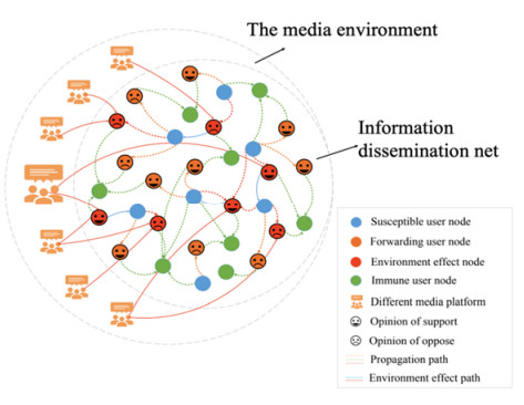
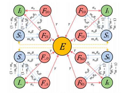
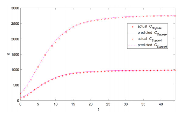
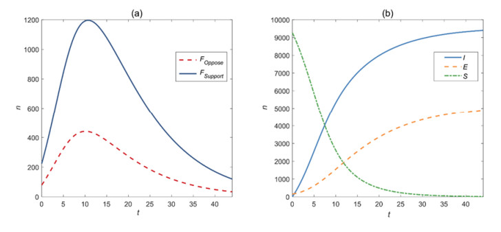
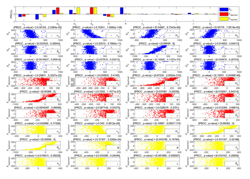
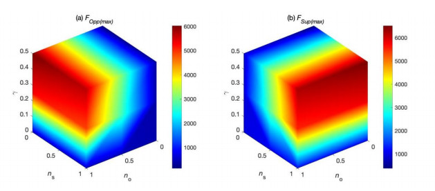
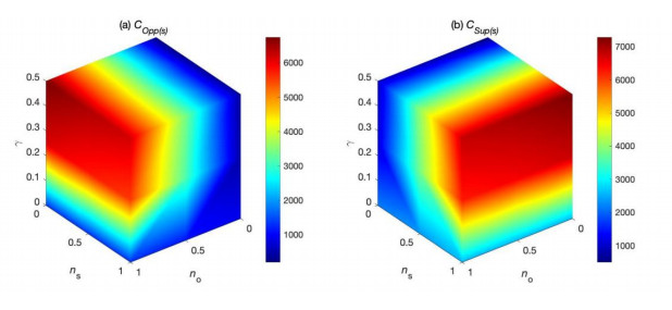
With the development of Internet technology, social media has gradually become an important platform where users can express opinions about hot events. Research on the mechanism of public opinion evolution is beneficial to guide the trend of opinions, making users' opinions change in a positive direction or reach a consensus among controversial crowds. To design effective strategies for public opinion management, we propose a dynamic opinion network susceptible-forwarding-immune model considering environmental factors (NET-OE-SFI), which divides the forwarding nodes into two types: support and opposition based on the real data of users. The NET-OE-SFI model introduces environmental factors from infectious diseases into the study of network information transmission, which aims to explore the evolution law of users' opinions affected by the environment. We attempt to combine the complex media environmental factors in social networks with users' opinion information to study the influence of environmental factors on the evolution of public opinion. Data fitting of real information transmission data fully demonstrates the validity of this model. We have also made a variety of sensitivity analysis experiments to study the influence of model parameters, contributing to the design of reasonable and effective strategies for public opinion guidance.

Keywords:

Citation: Fulian Yin, Jinxia Wang, Xinyi Jiang, Yanjing Huang, Qianyi Yang, Jianhong Wu. Modeling and analyzing an opinion network dynamics considering the environmental factor[J]. Mathematical Biosciences and Engineering, 2023, 20(9): 16866-16885. doi: 10.3934/mbe.2023752

Related Papers:

[1]	Jinbao Song, Xiaoya Zhu . Research on public opinion guidance of converging media based on AHP and transmission dynamics. Mathematical Biosciences and Engineering, 2021, 18(5): 6857-6886. doi: 10.3934/mbe.2021341
[2]	Elodie Yedomonhan, Chénangnon Frédéric Tovissodé, Romain Glèlè Kakaï . Modeling the effects of Prophylactic behaviors on the spread of SARS-CoV-2 in West Africa. Mathematical Biosciences and Engineering, 2023, 20(7): 12955-12989. doi: 10.3934/mbe.2023578
[3]	Fulian Yin, Xueying Shao, Jianhong Wu . Nearcasting forwarding behaviors and information propagation in Chinese Sina-Microblog. Mathematical Biosciences and Engineering, 2019, 16(5): 5380-5394. doi: 10.3934/mbe.2019268
[4]	Fulian Yin, Jiahui Lv, Xiaojian Zhang, Xinyu Xia, Jianhong Wu . COVID-19 information propagation dynamics in the Chinese Sina-microblog. Mathematical Biosciences and Engineering, 2020, 17(3): 2676-2692. doi: 10.3934/mbe.2020146
[5]	Xiaonan Chen, Suxia Zhang . An SEIR model for information propagation with a hot search effect in complex networks. Mathematical Biosciences and Engineering, 2023, 20(1): 1251-1273. doi: 10.3934/mbe.2023057
[6]	Bochuan Du, Pu Tian . Factorization in molecular modeling and belief propagation algorithms. Mathematical Biosciences and Engineering, 2023, 20(12): 21147-21162. doi: 10.3934/mbe.2023935
[7]	Qiao Xiang, Tianhong Huang, Qin Zhang, Yufeng Li, Amr Tolba, Isack Bulugu . A novel sentiment analysis method based on multi-scale deep learning. Mathematical Biosciences and Engineering, 2023, 20(5): 8766-8781. doi: 10.3934/mbe.2023385
[8]	Wei Hong, Yiting Gu, Linhai Wu, Xujin Pu . Impact of online public opinion regarding the Japanese nuclear wastewater incident on stock market based on the SOR model. Mathematical Biosciences and Engineering, 2023, 20(5): 9305-9326. doi: 10.3934/mbe.2023408
[9]	Wenjie Yang, Qianqian Zheng, Jianwei Shen, Linan Guan . Bifurcation and pattern dynamics in the nutrient-plankton network. Mathematical Biosciences and Engineering, 2023, 20(12): 21337-21358. doi: 10.3934/mbe.2023944
[10]	Yunyuan Gao, Zhen Cao, Jia Liu, Jianhai Zhang . A novel dynamic brain network in arousal for brain states and emotion analysis. Mathematical Biosciences and Engineering, 2021, 18(6): 7440-7463. doi: 10.3934/mbe.2021368

Abstract

1. Introduction

In ^[1], we distinguished the limit from the infinite sequence. In ^[2], we defined the Operator axioms to extend the traditional real number system. In ^[3], we promoted the research in the following areas:

1. We improved on the Operator axioms.

2. We defined the VE function and EV function. For clarity, we rename VE Function ^[3] to Prefix Function. For clarity, we rename EV Function ^[3] to Suffix Function.

3. We proved two theorems about the Prefix function and Suffix function.

The Operator axioms forms a new arithmetic axiom. The [,Definition 2.2] defines real number system on the basis of the logical calculus $\{ \Phi, \Psi \}$ . The [,] defines new operators according to the definition of number systems. Real operators naturally produce new equations such as $y = [x++++[1+1]]$ , $y = [[1+1]----x]$ , $y = [x////[1+1]]$ and so on. In other words, real operators extend the traditional mathematical models which are selected to describe various scientific rules. Operator axioms have included infinite operators, so no other operator can be added to them. This means the Operator axioms is a complete real number system. In fact, infinite operators imply the completeness.

Thus, real operators exhibit potential value as follows:

1. Real operators can give new equations and inequalities so as to precisely describe the relation of mathematical objects.

2. Real operators can give new equations and inequalities so as to precisely describe the relation of scientific objects.

So real operators help to describe complex scientific rules which are difficult described by traditional equations and have an enormous application potential.

As to the equations including real operators, engineering computation often need the approximate solutions reflecting an intuitive order relation and equivalence relation. Although the order relation and equivalence relation of real numbers are consistent, they are not as intuitive as those of base-b expansions. In practice, it is quicker to determine the order relation and equivalence relation of base-b expansions. So we introduce numerical computations to approximate real numbers with base-b expansions.

The numerical computations we proposed are not the best methods to approximate real numbers with base-b expansions, but the simple methods to approximate real numbers with base-b expansions. The compution complexity of the numerical computations we proposed could be promoted furtherly. However, we first prove that the Operator axioms can run on any modern computer. The numerical computation we proposed blends mathematics and computer science. Modern science depends on both the mathematics and the computer science. Arithmetic is the core of both the mathematics and the science. As a senior arithmetic, the Operator axioms will promote both the mathematics and the science in the future.

Theorem 1.1. Any positive number $\xi$ may be expressed as a limit of an infinite base-b expansion sequence

$\begin{eqnarray} \lim\limits_{n \to \infty} A_{1} A_{2} \cdots A_{s+1}.\ a_1 a_2 a_3 \cdots a_n, \end{eqnarray}$

(1.1)

where $0 \leq A_{1} < b, 0 \leq A_{2} < b, \cdots, 0 \leq a_{n} < b$ , not all A and a are 0, and an infinity of the $a_n$ are less than (b-1). If $\xi \geq 1$ , then $A_{1} \geq 0$ .

Proof. Let $[\xi]$ be the integral part of $\xi$ . Then we write

$\begin{eqnarray} \xi = [\xi] + x = X + x, \end{eqnarray}$

(1.2)

where $X$ is an integer and $0 \leq x < 1$ , and consider $X$ and $x$ separately.

If $X > 0$ and $b^{s} \leq x < b^{s+1}$ , and $A_1$ and $X_1$ are the quotient and remainder when $X$ is divided by $b^{s}$ , then $X = A_1 \cdot b^{s} + X_1$ , where $0 < A_1 = [b^{-s}X] < b$ , $0 \leq X_1 < b^s$ .

Similarly

$\begin{eqnarray*} X_1 = & A_2 \cdot b^{s-1} + X_2 & (0 \leq A_2 < b, 0 \leq X_2 < b^{s-1}), \\ X_2 = & A_3 \cdot b^{s-2} + X_3 & (0 \leq A_3 < b, 0 \leq X_3 < b^{s-2}), \\ \cdots & \cdots & \cdots \\ X_{s-1} = & A_s \cdot b + X_s & (0 \leq A_s < b, 0 \leq X_s < b), \\ X_s = & A_{s+1} & (0 \leq A_{s+1} < b). \end{eqnarray*}$

Thus $X$ may be expressed uniquely in the form

$\begin{eqnarray} X = A_1 \cdot b^s + A_2 \cdot b^{s-1} + \cdots + A_s \cdot b + A_{s+1}, \end{eqnarray}$

(1.3)

where every $A$ is one of 0, 1, $\cdots$ , (b-1), and $A_1$ is not 0. We abbreviate this expression to

$\begin{eqnarray} X = A_1 A_2 \cdots A_s A_{s+1}, \end{eqnarray}$

(1.4)

the ordinary representation of $X$ in base-b expansion notation.

Passing to $x$ , we write

$\begin{eqnarray*} & X = f_1 & (0 \leq f_1 < 1). \end{eqnarray*}$

We suppose that $a_1 = [b f_1]$ , so that

$\begin{eqnarray*} \frac{a_1}{b} \leq f_1 < \frac{a_1 + 1}{b}; \end{eqnarray*}$

$a_1$ is one of 0, 1, $\cdots$ , (b-1), and

$\begin{eqnarray*} a_1 = [b f_1], & b f_1 = a_1 + f_2 & (0 \leq f_2 < 1). \end{eqnarray*}$

Similarly, we define $a_2, a_3, \cdots$ by

$\begin{eqnarray*} a_2 = [b f_2], & b f_2 = a_2 + f_3 & (0 \leq f_3 < 1), \\ a_3 = [b f_3], & b f_3 = a_3 + f_4 & (0 \leq f_4 < 1), \\ \cdots & \cdots & \cdots \end{eqnarray*}$

Every $a_n$ is one of 0, 1, $\cdots$ , (b-1). Thus

$\begin{eqnarray} x = x_n + g_{n+1}, \end{eqnarray}$

(1.5)

where

$\begin{eqnarray} x_n = \frac{a_1}{b} + \frac{a_2}{b^2} + \cdots + \frac{a_n}{b^n}, \end{eqnarray}$

(1.6)

$\begin{eqnarray} 0 \leq g_{n+1} = \frac{f_{n+1}}{b^n} < \frac{1}{b^n}. \end{eqnarray}$

(1.7)

We thus define a base-b expansion $.a_1 a_2 a_3 \cdots a_n \cdots$ associated with $x$ . We call $a_1, a_2, \cdots$ the first, second, $\cdots$ digits of the base-b expansion.

Since $a_n < b$ , the series

$\begin{eqnarray} \sum\limits_{1}^{\infty} \frac{a_n}{b^n} \end{eqnarray}$

(1.8)

is convergent; and since $g_{n+1} \rightarrow 0$ , its sum is $x$ . We may therefore write

$\begin{eqnarray} x = .\ a_1 a_2 a_3 \cdots, \end{eqnarray}$

(1.9)

the right-hand side being an abbreviation for the series (1.8).

We now combine (1.2), (1.4), and (1.9) in the form

$\begin{eqnarray} \xi = X + x = A_1 A_2 \cdots A_s A_{s+1}.\ a_1 a_2 a_3 \cdots; \end{eqnarray}$

(1.10)

and the claim follows.

Theorem 1.1 implies that every real number has base-b expansions arbitrary close to it. So in numerical computations for the Operator axioms, all operands and outputs are denoted by base-b expansions to intuitively show the order relation and equivalence relation.

The paper is organized as follows. In Section 2, we define the operation order for all operations in the Operator axioms. In Section 3, we construct the numerical computations for binary operations. In Section 4, we define some concepts in the Operator axioms.

2. Operation Order

In the Operator axioms, the number '1' is the only base-b expansion while the others derive from the operation of two numbers and one operator. For example, the number " $[[1+[1+1]]----[1+1]]$ " derives from the operation of the number " $[1+[1+1]]$ ", the number " $[1+1]$ " and the real operator " $----$ ".

Definition 2.1. Numerical computation is a conversion from an operation to an approximate base-b expansion.

In general, an operation includes many binary operators. For example, the operation " $[[1+[1+1]]----[1+1]]$ " includes three " $+$ " and one " $----$ ". Since each operator produces a binary operation, $n$ operator in an operation will produce $n$ binary operations. It is better to compute all binary operations in an operation in order. The order is denoted as Operation Order.

[,§5.3.1] stores tradition operations as an expression tree and then applies traversal algorithm to evaluate the expression tree. Likewise, each operation of the Operator axioms can be stored as an expression tree in which each number '1' become a leaf node and each operator become an internal node. Then Operation Order is just the traversal order of the expression tree. In this paper, we choose inorder traversal as Operation Order. illustrates an expression tree for the number " $[[1+[1+1]]----[1+1]]$ ".

Figure 1. An expression tree for the number "

$[[1+[1+1]]----[1+1]]$ ".

DownLoad: Full-Size Img PowerPoint

It is supposed that the numerical computation applies base-10 expansions. Then the numerical computation for " $[[1+[1+1]]----[1+1]]$ " will proceed with the following Operation Order:

$\begin{eqnarray*} [[1+[1+1]]--[1+1]] & = & [[1+2]----[1+1]] \\ & = & [3----[1+1]] \\ & = & [3----2] \end{eqnarray*}$

In summary, every operation in the Operator axioms can divide into many binary operations by Operation Order. So numerical computations focus on the binary operations.

3. Numerical computations for binary operations

In ^[3], Operator axioms have expressed the real number system. In this section, "real number" refer to the real number deduced from Operator axioms ^[3].

3.1. Division of binary operations

According to the complexity of numerical computations, we divide binary operations into low operations, middle operations and high operations. Table 1 lists their elements in detail.

Table 1. Division of binary operations.

	Low operations	Middle operations	High operations
Operators	$+, ++, -, --, /, //$	$+++, ---, ///$	$++++, +++++, \cdots,$
			$----, -----, \cdots,$
			$////, /////, \cdots$

| Show Table

DownLoad: CSV

3.2. Numerical computations for low operations

In the Operator axioms, $/$ is equal to $-$ while $//$ is equal to $--$ . From a traditional viewpoint, the low operations " $+, ++, -, -$ " are equal to basic arithmetic operations " $+, \times, -, \div$ ". So numerical computations for low operations have been constructed in elementary arithmetic.

3.3. Numerical computations for middle operations

From a traditional viewpoint, $+++$ is an exponentiation operation, $---$ is a root-extraction operation and $///$ is a logarithm operation. In this subsection, we import the numerical computations for the middle operations " $+++, ---, ///$ " in [5,§23].

Let $e$ be Euler's number. It is supposed that $a \in \bigl(-\infty, +\infty\bigl)$ is a base-b expansion, $n \in Z$ and $k \in N$ . The numerical computation for $[e+++a]$ can be constructed with the Taylor-series expansion as follows.

$\begin{eqnarray*} [e+++a] & = & \left[ \lim\limits_{k \to +\infty} \left( \sum\limits_{n = 0}^{k} [[a+++n]--[n!]] \right) \right] \\ & \approx & [1 + [a--[1!]] + [[a+++2]--[2!]] + [[a+++3]--[3!]] + \cdots + \\ && [[a+++n]--[n!]] + \cdots] \end{eqnarray*}$

It is supposed that $a \in \bigl(0, +\infty\bigl)$ is a base-b expansion and $n \in Z$ . Let $b = [[a-1]--[a+1]]$ , then the numerical computation for $[a///e]$ can be constructed with the Taylor-series expansion as follows.

$\begin{eqnarray*} [a///e] & = &[[[1+b]--[1-b]]///e] \\ & = & \left[ 2++\left[ \lim\limits_{k \to +\infty} \left( \sum\limits_{n = 0}^{k} [[b+++[2n+1]]--[2n+1]] \right) \right] \right] \\ & \approx & [2++[b + [[b+++3]--3] + [[b+++5]--5] + \cdots + \\ && [[b+++[2n+1]]--[2n+1]] + \cdots]] \end{eqnarray*}$

It is supposed that $a$ and $b$ are two base-b expansions, where $a \in \bigl(0, +\infty\bigl)$ and $b \in \bigl(-\infty, +\infty\bigl)$ . Then the numerical computation for $[a+++b]$ can be divided and conquered with the identity $[a+++b] = [e+++[b++[a///e]]]$ .

It is supposed that $[a+++b]$ is a real number, where $a \in \bigl(-\infty, 0\bigl]$ and $b \in \bigl(-\infty, +\infty\bigl)$ are two base-b expansions. Then the numerical computation for $[a+++b]$ can always be equated with the basic numerical computations as above and the basic arithmetic operations in the axioms (OA.1) $\sim$ (OA.75).

3.4. Numerical computations for high operations

It is supposed that the constants $n, a_1, a_2, b_1, b_2, c_1, c_2, m \in N$ .

Zero can be equated with a fraction $[[1-1]--1]$ . Any non-zero base-b expansion can be equated with a fraction $[[1-1]\pm[a_1--a_2]]$ for $a_1, a_2 \in N$ .

It is supposed that the constant $d \in R$ with $[1-1] < d$ . It is supposed that the constant $e \in R$ with $1 < e$ . For clarity, we rename VE Function ^[3] to Prefix Function. For clarity, we rename EV Function ^[3] to Suffix Function.

Definition 3.1. [,Definition 3.1] Prefix Function is the function $f : \bigl[1, +\infty\bigl) \rightarrow R$ defined by $f(x) = [x+++\dot{e}d]$ .

Definition 3.2. [,Definition 3.2] Suffix Function is the function $f : R \rightarrow R$ defined by $f(x) = [e+++\dot{e}x]$ .

Definition 3.3. [3,Definition 3.3] Fundamental operator functions are Prefix Function and Suffix Function.

Theorem 3.4. [3,Theorem 3.4] The Prefix Function $f(x) = [x+++\dot{e}d]$ is continuous, unbounded and strictly increasing.

Theorem 3.5. [3,Theorem 3.5] The Suffix Function $f(x) = [e+++\dot{e}x]$ is continuous, unbounded and strictly increasing.

It is supposed that the constant $t, u, v \in R$ .

Definition 3.6. Root Equations are the equations such as $f(x) = t$ such that:

1. The function $f(x)$ is real and continuous on any closed interval $\bigl[u, v\bigl]$ in the domain;

2. The equation $f(x) = t$ has only one root on the above interval $\bigl[u, v\bigl]$ ;

[,TABLE PT2.3] lists common root-finding methods and their convergence conditions. When $a$ acts as the lower guess and $b$ acts as the upper guess, both the bisection method [,§5.2] and Brent's method [,§6.4] always converge and find the only root on $\bigl[u, v\bigl]$ . But Brent's method converges faster than the bisection method and thus acts as the main root-finding method for Root Equations.

In the following, we construct all numerical computations for high operations by induction. It is supposed that the constant $p_1 \in R$ with $1 \leq p_1$ . It is supposed that the constant $p_2 \in R$ . It is supposed that the constant $q_1 \in R$ with $1 \leq q_1$ . It is supposed that the constant $q_2 \in R$ with $[1-1] \leq q_2$ . It is supposed that the constant $r_1 \in R$ with $[1-1] < r_1$ . It is supposed that the constant $r_2 \in R$ with $1 < r_2$ . In the following, we approximate these constants with those fractions such as $[a_1--a_2]$ .

1. The numerical computations for the operations $[p_1++++p_2]$ , $[q_1----q_2]$ , $[r_1////r_2]$ are constructed.

(a) A numerical computation for $[[a_1--a_2]++++[b_1--b_2]]$ with $1 \leq [a_1--a_2]$ and $[1-1] \leq [b_1--b_2]$ can be constructed.

i. $[b_1--b_2] \leq 1$ .

$\begin{eqnarray*} (A1) & (\bar{c} = [[[a_1--a_2]-1]++[1+[1+1]]]) \wedge & \\ & (\bar{d} = [[[a_1--a_2]-1]++[1+1]]) \wedge \\ & (\bar{e} = [[b_1--b_2]+++[1+1]]) \wedge & \\ & (\bar{f} = [[b_1--b_2]+++[1+[1+1]]]) \wedge & \\ & ([[a_1--a_2]++++[b_1--b_2]] = & \\ & [[1+[\bar{c}++[\bar{e}+++1]]]-[\bar{d}++[\bar{f}+++1]]]) & \text{by (OA.83), (OA.28)} \\ (A2) & (\bar{c} = [[[a_1--a_2]-1]++[1+[1+1]]]) \wedge & \\ & (\bar{d} = [[[a_1--a_2]-1]++[1+1]]) \wedge \\ & (\bar{e} = [[b_1--b_2]+++[1+1]]) \wedge & \\ & (\bar{f} = [[b_1--b_2]+++[1+[1+1]]]) \wedge & \\ & ([[a_1--a_2]++++[b_1--b_2]] = & \\ & [[1+[\bar{c}++\bar{e}]]-[\bar{d}++\bar{f}]]) & \text{by (OA.83), (OA.62)} \\ \end{eqnarray*}$

ii. $1 < [b_1--b_2]$ .

$\begin{eqnarray*} (B1) & [[a_1--a_2]++++[b_1--b_2]] = & \\ & [[a_1--a_2]+++[[a_1--a_2]++++[[b_1--b_2]-1]]] & \text{by (OA.82)} \\ (B2) & \text{It is supposed that $ [1-1] \leq [[b_1--b_2]-n] $ and } & \\ & \text{$ [[b_1--b_2]-n] \leq 1 $. Let us distinguish these } & \\ & \text{$[a_1--a_2]$ with the subscripts } \{(1), (2), (3), \cdots\}. & \\ (B3) & \Rightarrow [[a_1--a_2]++++[b_1--b_2]] = & \\ & [[a_1--a_2]_{(1)}+++[[a_1--a_2]_{(2)}+++ \cdots \\ & [[a_1--a_2]_{n}+++ [[a_1--a_2]++++ & \\ & [[b_1--b_2]-n]] \cdots ]] & \text{by (OA.82), (B2)} \\ (B4) & (\bar{c} = [[[a_1--a_2]-1]++[1+[1+1]]]) \wedge & \\ & (\bar{d} = [[[a_1--a_2]-1]++[1+1]]) \wedge \\ & (\bar{e} = [[[b_1--b_2]-n]+++[1+1]]) \wedge & \\ & (\bar{f} = [[[b_1--b_2]-n]+++[1+[1+1]]]) \wedge & \\ & ([[a_1--a_2]++++[[b_1--b_2]-n]] = & \\ & [[1+[\bar{c}++\bar{e}]]-[\bar{d}++\bar{f}]]) & \text{by (B2), (A2)} \\ (B5) & \Rightarrow (\bar{c} = [[[a_1--a_2]-1]++[1+[1+1]]]) \wedge & \\ & (\bar{d} = [[[a_1--a_2]-1]++[1+1]]) \wedge \\ & (\bar{e} = [[[b_1--b_2]-n]+++[1+1]]) \wedge & \\ & (\bar{f} = [[[b_1--b_2]-n]+++[1+[1+1]]]) \wedge & \\ & ([[a_1--a_2]++++[b_1--b_2]] = & \\ & [[a_1--a_2]_{(1)}+++[[a_1--a_2]_{(2)}+++ \cdots \\ & [[a_1--a_2]_{n}+++ [[1+[\bar{c}++\bar{e}]]-[\bar{d}++\bar{f}]] \cdots ]]) & \text{by (B3), (B4)} \\ \end{eqnarray*}$

Then (A1) $\sim$ (A2) and (B1) $\sim$ (B4) have reduced one $++++$ operation to many $+++$ operations. Since §3.3 has constructed the numerical computation for $[[a_1--a_2]++++[b_1--b_2]]$ , (A1) $\sim$ (A2) and (B1) $\sim$ (B4) can achieve a numerical computation for $[[a_1--a_2]++++[b_1--b_2]]$ .

(b) A numerical computation for $[[a_1--a_2]----[b_1--b_2]]$ with $1 \leq [a_1--a_2]$ and $[1-1] < [b_1--b_2]$ can be constructed.

The numerical computation for $[[a_1--a_2]----[b_1--b_2]]$ is equated with the numerical root finding of the equation $x = [[a_1--a_2]----[b_1--b_2]]$ .

$\begin{eqnarray*} (A1) & x = [[a_1--a_2]----[b_1--b_2]] & \\ (A2) & \Rightarrow [x++++[b_1--b_2]] = & \\ & [[[a_1--a_2]----[b_1--b_2]] & \\ & ++++[b_1--b_2]] & \text{by (OA.108)} \\ (A3) & \Rightarrow [x++++[b_1--b_2]] = [a_1--a_2] & \text{by (OA.79), (OA.24), } \\ && \text{(OA.25)} \end{eqnarray*}$

According to (OA.37) $\sim$ (OA.40), the function $f(x) = [x++++[b_1--b_2]]$ is defined on the domain $\bigl[1, +\infty\bigl)$ . Theorem 3.4 implies that we can iteratively increase $v$ by step 1 from $v = 1$ until $[a_1--a_2] < [v++++[b_1--b_2]]$ holds.

Theorem 3.4 implies that $f(x) = [x++++[b_1--b_2]]$ is continuous on the domain $\bigl[1, v\bigl]$ . (OA.75) derives that $[1++++[b_1--b_2]] = 1$ . So (OA.95) derives that $[1++++[b_1--b_2]] \leq [a_1--a_2]$ . In summary, both $[1++++[b_1--b_2]] \leq [a_1--a_2]$ and $[a_1--a_2] < [v++++[b_1--b_2]]$ hold.

Then Intermediate Value Theorem derives that the equation $[x++++[b_1--b_2]] = [a_1--a_2]$ has only one root on the domain $\bigl[1, v\bigl]$ . Since Theorem 3.4 implies that the equation $[x++++[b_1--b_2]] = [a_1--a_2]$ has no root on the domain $\bigl(v, +\infty\bigl)$ , the equation $[x++++[b_1--b_2]] = [a_1--a_2]$ has only one root on the domain $\bigl[[1-1], +\infty\bigl)$ . Since the equation $[x++++[b_1--b_2]] = [a_1--a_2]$ belongs to Root Equations, Brent's method can find the only root of the equation and constructs the numerical computation for $[[a_1--a_2]----[b_1--b_2]]$ .

(c) A numerical computation for $[[a_1--a_2]////[b_1--b_2]]$ with $1 \leq [a_1--a_2]$ and with $1 < [b_1--b_2]$ can be constructed.

The numerical computation for $[[a_1--a_2]////[b_1--b_2]]$ is equated with the numerical root finding of the equation $x = [[a_1--a_2]////[b_1--b_2]]$ .

$\begin{eqnarray*} (A1) & x = [[a_1--a_2]////[b_1--b_2]] & \\ (A2) & [1-1] < [[a_1--a_2]////[b_1--b_2]] & \text{by (OA.33)} \\ (A3) & \Rightarrow 1 < [[b_1--b_2]++++ & \\ & [[a_1--a_2]////[b_1--b_2]]] & \text{by (OA.37), (OA.72)} \\ (A4) & \Rightarrow ([[b_1--b_2]++++ & \\ & [[a_1--a_2]////[b_1--b_2]]]) & \text{by (OA.90)} \\ (A5) & \Rightarrow [[b_1--b_2]++++x] = & \\ & [[b_1--b_2]++++ & \\ & [[a_1--a_2]////[b_1--b_2]]] & \text{by (OA.105)} \\ (A6) & \Rightarrow [[b_1--b_2]++++x] = [a_1--a_2] & \text{by (OA.80), (OA.104)} \end{eqnarray*}$

According to (OA.37) $\sim$ (OA.40) and (OA.73), the function $f(x) = [[b_1--b_2]++++x]$ is defined on the domain $\bigl(-\infty, +\infty\bigl)$ . Theorem 3.5 implies that we can iteratively decrease $u$ by step 1 from $u = 1$ until $[[b_1--b_2]++++u] < [a_1--a_2]$ holds. Theorem 3.5 also implies that we can iteratively increase $v$ by step 1 from $v = 1$ until $[a_1--a_2] < [[b_1--b_2]++++v]$ holds.

Theorem 3.5 implies that $f(x) = [[b_1--b_2]++++x]$ is continuous on the domain $\bigl(-\infty, +\infty\bigl)$ . In summary, both $[[b_1--b_2]++++u] < [a_1--a_2]$ and $[a_1--a_2] < [[b_1--b_2]++++v]$ hold.

Then Intermediate Value Theorem derives that the equation $[[b_1--b_2]++++x] = [a_1--a_2]$ has only one root on the domain $\bigl[u, v\bigl]$ . Since Theorem 3.5 implies that the equation $[[b_1--b_2]++++x] = [a_1--a_2]$ has no root on the domains $\bigl(-\infty, u\bigl)$ and $\bigl(v, +\infty\bigl)$ , the equation $[[b_1--b_2]++++x] = [a_1--a_2]$ has only one root on the domain $\bigl[u, v\bigl]$ . Since the equation $[[b_1--b_2]++++x] = [a_1--a_2]$ belongs to Root Equations, Brent's method can find the only root of the equation and constructs the numerical computation for $[[a_1--a_2]////[b_1--b_2]]$ .

2. If the numerical computations for $[p_1+++\dot{e}p_2]$ , $[q_1---\dot{f}q_2]$ , $[r_1///\dot{g}r_2]$ have been constructed, then the numerical computations for $[p_1++++\dot{e}p_2]$ , $[q_1----\dot{f}q_2]$ , $[r_1////\dot{g}r_2]$ can also be constructed.

According to (OA.19), the symbol ' $e$ ' represents some successive ' $+$ '—" $+ \cdots +$ ". According to (OA.20), the symbol ' $f$ ' represents some successive ' $-$ '—" $- \cdots -$ ". According to (OA.21), the symbol ' $g$ ' represents some successive ' $/$ '—" $/ \cdots /$ ".

(a) A numerical computation for $[[a_1--a_2]++++\dot{e}[b_1--b_2]]$ with $1 \leq [a_1--a_2]$ and $[1-1] \leq [b_1--b_2]$ can be constructed.

i. $[b_1--b_2] \leq 1$ .

ii. $1 < [b_1--b_2]$ .

$\begin{eqnarray*} (B1) & [[a_1--a_2]++++\dot{e}[b_1--b_2]] = & \\ & [[a_1--a_2]+++\dot{e}[[a_1--a_2]++++\dot{e}[[b_1--b_2]-1]]] & \text{by (OA.82)} \\ (B2) & \text{It is supposed that $ [1-1] \leq [[b_1--b_2]-n] $ and } & \\ & \text{$ [[b_1--b_2]-n] \leq 1 $. Let us distinguish these } & \\ & \text{$[a_1--a_2]$ with the subscripts } \{(1), (2), (3), \cdots\}. & \\ (B3) & \Rightarrow [[a_1--a_2]++++\dot{e}[b_1--b_2]] = & \\ & [[a_1--a_2]_{(1)}+++\dot{e}[[a_1--a_2]_{(2)}+++\dot{e} \cdots \\ & [[a_1--a_2]_{n}+++\dot{e} [[a_1--a_2]++++\dot{e} & \\ & [[b_1--b_2]-n]] \cdots ]] & \text{by (OA.82), (B2)} \\ (B4) & (\bar{c} = [[[a_1--a_2]-1]++[1+[1+1]]]) \wedge & \\ & (\bar{d} = [[[a_1--a_2]-1]++[1+1]]) \wedge \\ & (\bar{e} = [[[b_1--b_2]-n]+++[1+1]]) \wedge & \\ & (\bar{f} = [[[b_1--b_2]-n]+++[1+[1+1]]]) \wedge & \\ & ([[a_1--a_2]++++\dot{e}[[b_1--b_2]-n]] = & \\ & [[1+[\bar{c}++\bar{e}]]-[\bar{d}++\bar{f}]]) & \text{by (B3), (A1)} \\ (B5) & \Rightarrow (\bar{c} = [[[a_1--a_2]-1]++[1+[1+1]]]) \wedge & \\ & (\bar{d} = [[[a_1--a_2]-1]++[1+1]]) \wedge \\ & (\bar{e} = [[[b_1--b_2]-n]+++[1+1]]) \wedge & \\ & (\bar{f} = [[[b_1--b_2]-n]+++[1+[1+1]]]) \wedge & \\ & ([[a_1--a_2]++++\dot{e}[b_1--b_2]] = & \\ & [[a_1--a_2]_{(1)}+++\dot{e}[[a_1--a_2]_{(2)}+++\dot{e} \cdots \\ & [[a_1--a_2]_{n}+++\dot{e} [[1+[\bar{c}++\bar{e}]]-[\bar{d}++\bar{f}]] \cdots ]]) & \text{by (B3), (B4)} \\ \end{eqnarray*}$

Then (A1) and (B1) $\sim$ (B5) have reduced one $++++\dot{e}$ operation to many $+++\dot{e}$ operations. Since the numerical computation for $[[a_1--a_2]+++\dot{e}[b_1--b_2]]$ has been supposed to be constructed, (A1) and (B1) $\sim$ (B5) can achieve a numerical computation for $[[a_1--a_2]++++\dot{e}[b_1--b_2]]$ .

(b) A numerical computation for $[[a_1--a_2]----\dot{f}[b_1--b_2]]$ with $1 \leq [a_1--a_2]$ and $[1-1] < [b_1--b_2]$ can be constructed.

The numerical computation for $[[a_1--a_2]----\dot{f}[b_1--b_2]]$ is equated with the numerical root finding of the equation $x = [[a_1--a_2]----\dot{f}[b_1--b_2]]$ .

$\begin{eqnarray*} (A1) & x = [[a_1--a_2]----\dot{f}[b_1--b_2]] & \\ (A2) & \Rightarrow [x++++\dot{e}[b_1--b_2]] = & \\ & [[[a_1--a_2]----i[b_1--b_2]] & \\ & ++++h[b_1--b_2]] & \text{by (OA.105)} \\ (A3) & \Rightarrow [x++++\dot{e}[b_1--b_2]] = [a_1--a_2] & \text{by (OA.78), (OA.24), } \\ && \text{(OA.25)} \end{eqnarray*}$

According to (OA.37) $\sim$ (OA.40), the function $f(x) = [x++++\dot{e}[b_1--b_2]]$ is defined on the domain $\bigl[1, +\infty\bigl)$ . Theorem 3.4 implies that we can iteratively increase $v$ by step 1 from $v = 1$ until $[a_1--a_2] < [v++++\dot{e}[b_1--b_2]]$ holds.

Theorem 3.4 implies that $f(x) = [x++++\dot{e}[b_1--b_2]]$ is continuous on the domain $\bigl[1, v\bigl]$ . (OA.75) derives that $[1++++\dot{e}[b_1--b_2]] = 1$ . So (OA.95) derives that $[1++++\dot{e}[b_1--b_2]] \leq [a_1--a_2]$ . In summary, both $[1++++\dot{e}[b_1--b_2]] \leq [a_1--a_2]$ and $[a_1--a_2] < [v++++\dot{e}[b_1--b_2]]$ hold.

Then Intermediate Value Theorem derives that the equation $[x++++\dot{e}[b_1--b_2]] = [a_1--a_2]$ has only one root on the domain $\bigl[1, v\bigl]$ . Since Theorem 3.4 implies that the equation $[x++++\dot{e}[b_1--b_2]] = [a_1--a_2]$ has no root on the domain $\bigl(v, +\infty\bigl)$ , the equation $[x++++\dot{e}[b_1--b_2]] = [a_1--a_2]$ has only one root on the domain $\bigl[[1-1], +\infty\bigl)$ . Since the equation $[x++++\dot{e}[b_1--b_2]] = [a_1--a_2]$ belongs to Root Equations, Brent's method can find the only root of the equation and constructs the numerical computation for $[[a_1--a_2]----\dot{f}[b_1--b_2]]$ .

(c) A numerical computation for $[[a_1--a_2]////\dot{g}[b_1--b_2]]$ with $1 \leq [a_1--a_2]$ and with $1 < [b_1--b_2]$ can be constructed.

The numerical computation for $[[a_1--a_2]////\dot{g}[b_1--b_2]]$ is equated with the numerical root finding of the equation $x = [[a_1--a_2]////\dot{g}[b_1--b_2]]$ .

$\begin{eqnarray*} (A1) & x = [[a_1--a_2]////\dot{g}[b_1--b_2]] & \\ (A2) & [1-1] < [[a_1--a_2]////\dot{g}[b_1--b_2]] & \text{by (OA.33)} \\ (A3) & \Rightarrow 1 < [[b_1--b_2]++++h & \\ & [[a_1--a_2]////j[b_1--b_2]]] & \text{by (OA.37), (OA.72)} \\ (A4) & \Rightarrow ([[b_1--b_2]++++h & \\ & [[a_1--a_2]////j[b_1--b_2]]]) & \text{by (OA.90)} \\ (A5) & \Rightarrow [[b_1--b_2]++++\dot{e}x] = & \\ & [[b_1--b_2]++++h & \\ & [[a_1--a_2]////j[b_1--b_2]]] & \text{by (OA.105)} \\ (A6) & \Rightarrow [[b_1--b_2]++++\dot{e}x] = [a_1--a_2] & \text{by (OA.80), (OA.104)} \end{eqnarray*}$

According to (OA.37) $\sim$ (OA.40) and (OA.73), the function $f(x) = [[b_1--b_2]++++\dot{e}x]$ is defined on the domain $\bigl(-\infty, +\infty\bigl)$ . Theorem 3.5 implies that we can iteratively decrease $u$ by step 1 from $u = 1$ until $[[b_1--b_2]++++\dot{e}u] < [a_1--a_2]$ holds. Theorem 3.5 also implies that we can iteratively increase $v$ by step 1 from $v = 1$ until $[a_1--a_2] < [[b_1--b_2]++++\dot{e}v]$ holds.

Theorem 3.5 implies that $f(x) = [[b_1--b_2]++++\dot{e}x]$ is continuous on the domain $\bigl(-\infty, +\infty\bigl)$ . In summary, both $[[b_1--b_2]++++\dot{e}u] < [a_1--a_2]$ and $[a_1--a_2] < [[b_1--b_2]++++\dot{e}v]$ hold.

Then Intermediate Value Theorem derives that the equation $[[b_1--b_2]++++\dot{e}x] = [a_1--a_2]$ has only one root on the domain $\bigl[u, v\bigl]$ . Since Theorem 3.5 implies that the equation $[[b_1--b_2]++++\dot{e}x] = [a_1--a_2]$ has no root on the domains $\bigl(-\infty, u\bigl)$ and $\bigl(v, +\infty\bigl)$ , the equation $[[b_1--b_2]++++\dot{e}x] = [a_1--a_2]$ has only one root on the domain $\bigl[u, v\bigl]$ . Since the equation $[[b_1--b_2]++++\dot{e}x] = [a_1--a_2]$ belongs to Root Equations, Brent's method can find the only root of the equation and constructs the numerical computation for $[[a_1--a_2]////\dot{g}[b_1--b_2]]$ .

3. By induction, the numerical computations for $[p_1+++++p_2]$ , $[p_1++++++p_2]$ , $[p_1+++++++p_2]$ , $\cdots$ , $[q_1-----q_2]$ , $[q_1------q_2]$ , $[q_1-------q_2]$ , $\cdots$ , $[r_1/////r_2]$ , $[r_1//////r_2]$ , $[r_1///////r_2]$ , $\cdots$ can all be constructed.

4. Some concepts in the Operator axioms

We define some replacements for the notations of the Operator axioms, as is shown in Table 2.

Table 2. Replacements of notations.

Replacement	Notation in Operator axioms
$+'$	$\dot{e}$
$-'$	$\dot{f}$
$/'$	$\dot{j}$
$+'_1$	$+$
$+'_2$	$++$
$+'_3$	$+++$
$+'_n$	$\underbrace{++\cdots+}_{n}$
$-'_1$	$-$
$-'_2$	$--$
$-'_3$	$---$
$-'_n$	$\underbrace{--\cdots-}_{n}$
$/'_1$	$/$
$/'_2$	$//$
$/'_3$	$///$
$/'_n$	$\underbrace{//\cdots/}_{n}$

| Show Table

DownLoad: CSV

The notation $+'$ can be replaced by any element of the set $\{ +, ++, +++, ++++, \cdots \}$ . The notation $-'$ can be replaced by any element of the set $\{ -, --, ---, ----, \cdots \}$ . The notation $/'$ can be replaced by any element of the set $\{ /, //, ///, ////, \cdots \}$ .

We define the pronunciations for some expressions in the Operator axioms, as is shown in Table 3.

Table 3. Pronunciations for some expressions.

Expression	Pronunciation
$+'$	addote
$-'$	subote
$/'$	logote
$a +'_n b$	a addote n to b
$a -'_n b$	a subote n to b
$a /'_n b$	a logote n to b

| Show Table

DownLoad: CSV

We divide the real operators into an ordered level with the natural numbers. Table 4 lists the levels of the real operators in detail.

Table 4. Level of operators.

Level	Operators
1	$+'_1, -'_1, /'_1$
2	$+'_2, -'_2, /'_2$
3	$+'_3, -'_3, /'_3$
$\cdots$	$\cdots$
n	$+'_n, -'_n, /'_n$

| Show Table

DownLoad: CSV

The order of real operators is listed as follows:

level-1 $<$ level-2 $<$ level-3 $< \cdots$ $<$ level-n

We define the operations of real operators as follows.

Definition 4.1. Complete Operations are all the binary operations of real operators.

According to the Definition 4.1, all operations such as $a +'_n b$ , $a -'_n b$ , $a /'_n b$ compose the complete operations.

Conflict of interest

The author declares no conflict of interest.

References

[1]	S. Galam, Modelling rumors: the no plane Pentagon French hoax case, Physica A, 320 (2003), 571–580. https://doi.org/10.1016/S0378-4371(02)01582-0 doi: 10.1016/S0378-4371(02)01582-0
[2]	J. Zhou, Z. Liu, B. Li, Influence of network structure on rumor propagation, Phys. Lett. A, 368 (2007), 458–463. https://doi.org/10.1016/j.physleta.2007.01.094 doi: 10.1016/j.physleta.2007.01.094
[3]	B. Zhang, X. Guan, M. J. Khan, Y. Zhou, A time-varying propagation model of hot topic on BBS sites and Blog networks, Inf. Sci., 187 (2012), 15–32. https://doi.org/10.1016/j.ins.2011.09.025 doi: 10.1016/j.ins.2011.09.025
[4]	M. E. J. Newman, Fast algorithm for detecting community structure in networks, Phys. Rev. E, 69 (2004), 066133. https://doi.org/10.1103/PhysRevE.69.066133 doi: 10.1103/PhysRevE.69.066133
[5]	A. Mislove, H. S. Koppula, K. P. Gummadi, P. Druschel, B. Bhattacharjee, Growth of the flickr social network, in Proceedings of the First Workshop on Online Social Networks, (2008), 25–30. https://doi.org/10.1145/1397735.1397742
[6]	Y. Bao, C. Yi, Y. Xue, Y. Dong, Precise modeling rumor propagation and control strategy on social networks, in Applications of Social Media and Social Network Analysis, (2015), 77–102. https://doi.org/10.1007/978-3-319-19003-7_5
[7]	J. Yi, P. Liu, X. Tang, W. Liu, Improved SIR advertising spreading model and its effectiveness in social network, Procedia Comput. Sci., 129 (2018), 215–218. https://doi.org/10.1016/j.procs.2018.03.044 doi: 10.1016/j.procs.2018.03.044
[8]	N. Liu, H. An, X. Gao, H. Li, X. Hao, Breaking news dissemination in the media via propagation behavior based on complex network theory, Physica A, 453 (2016), 44–54. https://doi.org/10.1016/j.physa.2016.02.046 doi: 10.1016/j.physa.2016.02.046
[9]	L. Yang, Z. Li, A. Giua, Containment of rumor spread in complex social networks, Inf. Sci., 506 (2020), 113–130. https://doi.org/10.1016/j.ins.2019.07.055 doi: 10.1016/j.ins.2019.07.055
[10]	X. Liu, D. He, Nonlinear dynamic information propagation mathematic modeling and analysis based on microblog social network, Social Network Anal. Min., 10 (2020), 1–12. https://doi.org/10.1007/s13278-020-00700-4 doi: 10.1007/s13278-020-00700-4
[11]	S. Ai, S. Hong, X. Zheng, Y. Wang, X. Liu, CSRT rumor spreading model based on complex network, Int. J. Intell. Syst., 36 (2021), 1903–1913. https://doi.org/10.1002/int.22365 doi: 10.1002/int.22365
[12]	R. Sun, W. B. Luo, Rumor propagation model for complex network with non-uniform propagation rates, Appl. Mech. Mater., 596 (2014), 868–872. https://doi.org/10.4028/www.scientific.net/AMM.596.868 doi: 10.4028/www.scientific.net/AMM.596.868
[13]	A. Singh, Y. N. Singh, Rumor dynamics in weighted scale-free networks with degree correlations, J. Complex Networks, 3 (2015), 450–468. https://doi.org/10.1093/comnet/cnu047 doi: 10.1093/comnet/cnu047
[14]	F. Nian, K. Gao, Evolution of node impact based on secondary propagation, Mod. Phys. Lett. B, 34 (2020), 2050027. https://doi.org/10.1142/S021798492050027X doi: 10.1142/S021798492050027X
[15]	M. Zhang, S. Qin, X. Zhu, Information diffusion under public crisis in BA scale-free network based on SEIR model-Taking COVID-19 as an example, Physica A, 571 (2021), 125848. https://doi.org/10.1016/j.physa.2021.125848 doi: 10.1016/j.physa.2021.125848
[16]	Z, Dang, L. Li, H. Peng, J. Zhang, The behavior propagation and confrontation competition model based on information energy, Int. J. Mod. Phys. B, 35 (2021), 2150281. https://doi.org/10.1142/S0217979221502817 doi: 10.1142/S0217979221502817
[17]	H. Wang, J. M. Moore, M. Small, J. Wang, H. Yang, C. Gu, Epidemic dynamics on higher-dimensional small world networks, Appl. Math. Comput., 421 (2022), 126911. https://doi.org/10.1016/j.amc.2021.126911 doi: 10.1016/j.amc.2021.126911
[18]	K. Sznajd-Weron, J. Sznajd, Opinion evolution in closed community, Int. J. Mod. Phys. C, 11 (2000), 1157–1165. https://doi.org/10.1142/S0129183100000936 doi: 10.1142/S0129183100000936
[19]	S. Galam, Minority opinion spreading in random geometry, Eur. Phys. J. B, 25 (2002), 403–406. https://doi.org/10.1140/epjb/e20020045 doi: 10.1140/epjb/e20020045
[20]	G. Deffuant, D. Neau, F. Amblard, G. Weisbuch, Mixing beliefs among interacting agents, Adv. Complex Syst., 3 (2000), 87–98. https://doi.org/10.1142/S0219525900000078 doi: 10.1142/S0219525900000078
[21]	R. Hegselmann, U. Krause, Opinion dynamics and bounded confidence models, analysis and simulation, J. Artif. Soc. Social Simul., 5 (2002), 1–2.
[22]	H. Zhu, Y. Kong, J. Wei, J. Ma, Effect of users' opinion evolution on information diffusion in online social networks, Physica A, 492 (2018), 2034–2045. https://doi.org/10.1016/j.physa.2017.11.121 doi: 10.1016/j.physa.2017.11.121
[23]	Q. Li, Y. J. Du, Z. Y. Li, J. R. Hu, R. L. Hu, B. Y. Lv, et al., HK-SEIR model of public opinion evolution based on communication factors, Eng. Appl. Artif. Intell., 100 (2021), 104192. https://doi.org/10.1016/j.engappai.2021.104192 doi: 10.1016/j.engappai.2021.104192
[24]	D. Liang, B. Yi, Z. Xu, Opinion dynamics based on infectious disease transmission model in the non-connected context of Pythagorean fuzzy trust relationship, J. Oper. Res. Soc., 72 (2021), 2783–2803. https://doi.org/10.1080/01605682.2020.1821585 doi: 10.1080/01605682.2020.1821585
[25]	C. Wang, Dynamics of conflicting opinions considering rationality, Physica A, 560 (2020), 125160. https://doi.org/10.1016/j.physa.2020.125160 doi: 10.1016/j.physa.2020.125160
[26]	K. Mitsutsuji, S. Yamakage, The dual attitudinal dynamics of public opinion: an agent-based reformulation of LF Richardson's war-moods model, Qual. Quant., 54 (2020), 439–461. https://doi.org/10.1007/s11135-019-00938-x doi: 10.1007/s11135-019-00938-x
[27]	S. Chen, D. H. Glass, M. McCartney, Characteristics of successful opinion leaders in a bounded confidence model, Physica A, 449 (2016), 426–436. https://doi.org/10.1016/j.physa.2015.12.107 doi: 10.1016/j.physa.2015.12.107
[28]	Y. Zhao, G. Kou, Y. Peng, Y. Chen, Understanding influence power of opinion leaders in e-commerce networks: An opinion dynamics theory perspective, Inf. Sci., 426 (2018), 131–147. https://doi.org/10.1016/j.ins.2017.10.031 doi: 10.1016/j.ins.2017.10.031
[29]	Z. Feng, J. Velasco-Hernandez, B. Tapia-Santos, A mathematical model for coupling within-host and between-host dynamics in an environmentally-driven infectious disease, Math. Biosci., 241 (2013), 49–55. https://doi.org/10.1016/j.mbs.2012.09.004 doi: 10.1016/j.mbs.2012.09.004
[30]	A. Meiksin, Dynamics of COVID-19 transmission including indirect transmission mechanisms: a mathematical analysis, Epidemiol. Infect., 148 (2020), e257. https://doi.org/10.1017/S0950268820002563 doi: 10.1017/S0950268820002563
[31]	R. I. Joh, H. Wang, H. Weiss, J. S. Weitz, Dynamics of indirectly transmitted infectious diseases with immunological threshold, Bull. Math. Biol., 71 (2009), 845–862. https://doi.org/10.1007/s11538-008-9384-4 doi: 10.1007/s11538-008-9384-4
[32]	Z. Shuai, P. Van den Driessche, Global dynamics of cholera models with differential infectivity, Math. Biosci., 234 (2011), 118–126. https://doi.org/10.1016/j.mbs.2011.09.003 doi: 10.1016/j.mbs.2011.09.003
[33]	S. Liao, J. Wang, Global stability analysis of epidemiological models based on Volterra–Lyapunov stable matrices, Chaos, Solitons Fractals, 45 (2012), 966–977. https://doi.org/10.1016/j.chaos.2012.03.009 doi: 10.1016/j.chaos.2012.03.009
[34]	J. F. David, S. A. Iyaniwura, M. J. Ward, F. Brauer, A novel approach to modelling the spatial spread of airborne diseases: an epidemic model with indirect transmission, Math. Biosci. Eng., 17 (2020), 3294–3328. https://doi.org/10.3934/mbe.2020188 doi: 10.3934/mbe.2020188
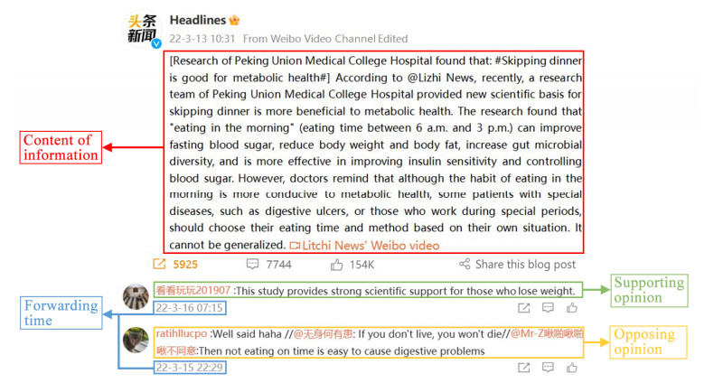
[35]	F. Yin, X. Shao, J. Wu, Nearcasting forwarding behaviors and information propagation in Chinese Sina-Microblog, Math. Biosci. Eng., 16 (2019), 5380–5394. https://doi.org/10.3934/mbe.2019268 doi: 10.3934/mbe.2019268

This article has been cited by:

1.	Jakob Schneider, Ksenia Korshunova, Zeineb Si Chaib, Alejandro Giorgetti, Mercedes Alfonso-Prieto, Paolo Carloni, Ligand Pose Predictions for Human G Protein-Coupled Receptors: Insights from the Amber-Based Hybrid Molecular Mechanics/Coarse-Grained Approach, 2020, 60, 1549-9596, 5103, 10.1021/acs.jcim.0c00661
2.	Stefano Capaldi, Eda Suku, Martina Antolini, Mattia Di Giacobbe, Alejandro Giorgetti, Mario Buffelli, Allosteric sodium binding cavity in GPR3: a novel player in modulation of Aβ production, 2018, 8, 2045-2322, 10.1038/s41598-018-29475-7
3.	Jinan Wang, Yinglong Miao, 2019, 116, 9780128155615, 397, 10.1016/bs.apcsb.2018.11.011
4.	Filippo Baldessari, Riccardo Capelli, Paolo Carloni, Alejandro Giorgetti, Coevolutionary data-based interaction networks approach highlighting key residues across protein families: The case of the G-protein coupled receptors, 2020, 18, 20010370, 1153, 10.1016/j.csbj.2020.05.003

Reader Comments

Your name:*

Email:*
© 2023 the Author(s), licensee AIMS Press. This is an open access article distributed under the terms of the Creative Commons Attribution License (http://creativecommons.org/licenses/by/4.0)