Frequency hopping signal detection based on optimized generalized S transform and ResNet

Chun Li; Ying Chen; Zhijin Zhao; Chun Li; Ying Chen; Zhijin Zhao

doi:10.3934/mbe.2023573

Mathematical Biosciences and Engineering

2023, Volume 20, Issue 7: 12843-12863. doi: 10.3934/mbe.2023573

Previous Article Next Article

Research article Special Issues

Frequency hopping signal detection based on optimized generalized S transform and ResNet

School of Communication Engineering, Hangzhou Dianzi University, Hangzhou 310018, China

Academic Editor: Danilo Pelusi

Received: 09 March 2023 Revised: 11 May 2023 Accepted: 22 May 2023 Published: 02 June 2023

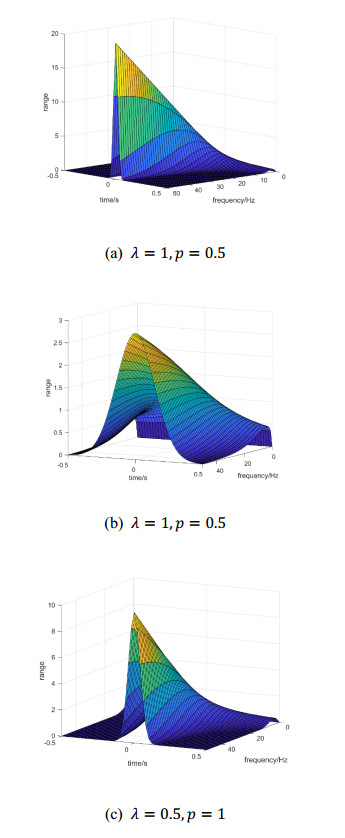
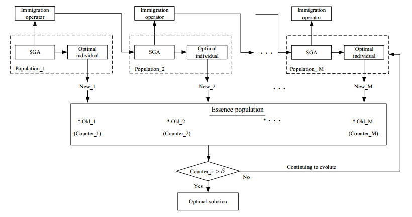
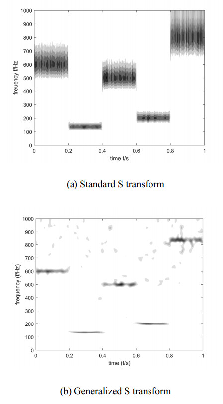
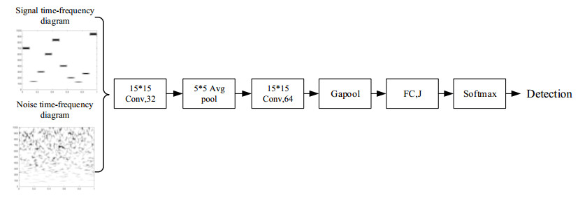
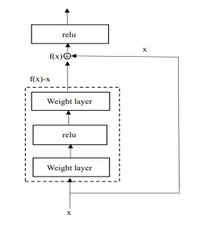
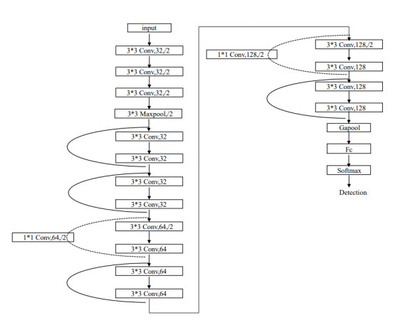
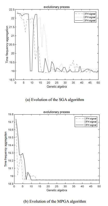
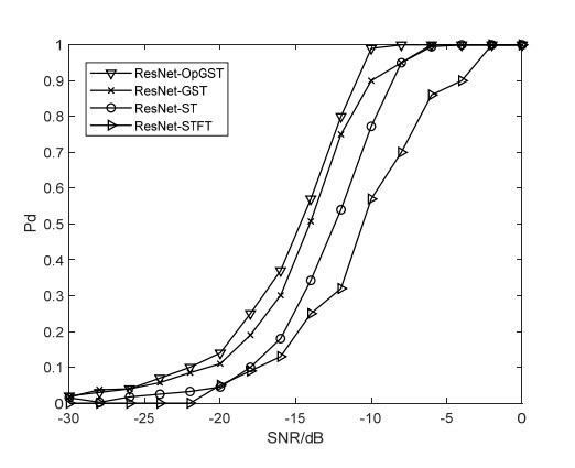
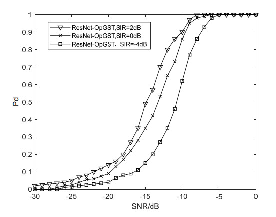
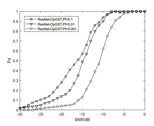
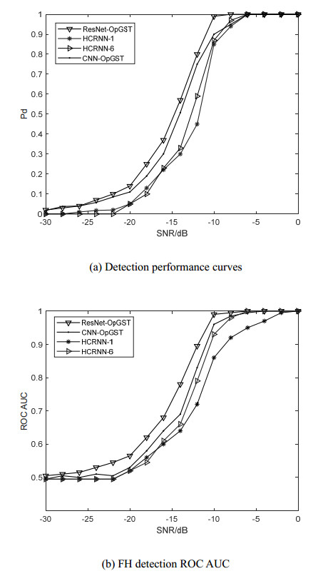
The performance of traditional frequency hopping signal detection methods based on time frequency analysis is limited by the tradeoff of time-frequency resolution and spectrum leakage. Machine learning-based frequency hopping signal detection techniques have a high level of complexity. Therefore, this paper proposes a residual network and the optimized generalized S transform to detect frequency hopping signals. First, based on the time-frequency aggregation measure, the generalized S transform parameters $ \lambda $ and $ p $ are optimized using a multi-population genetic algorithm. Second, the optimized generalized S transform is used to determine a signal's time-frequency spectrum, which is then normalized to make this robust to noise power uncertainty. Finally, a residual network structure is designed which receives the time-frequency spectrum. To detect frequency hopping signals, the network automatically learns the time-frequency properties of signals and noise. Simulated findings indicate that the multi-population genetic algorithm not only increases optimization efficiency when compared to a regular genetic algorithm, but also has faster convergence and more stable optimization results. Compared with a hybrid convolutional network/recurrent neural network algorithm, the proposed technique is better at detection and has less computational and storage complexity.
- frequency hopping signal detection,
- generalized S transform,
- genetic algorithm,
- convolutional neural network
Citation: Chun Li, Ying Chen, Zhijin Zhao. Frequency hopping signal detection based on optimized generalized S transform and ResNet[J]. Mathematical Biosciences and Engineering, 2023, 20(7): 12843-12863. doi: 10.3934/mbe.2023573

Related Papers:

Abstract

The performance of traditional frequency hopping signal detection methods based on time frequency analysis is limited by the tradeoff of time-frequency resolution and spectrum leakage. Machine learning-based frequency hopping signal detection techniques have a high level of complexity. Therefore, this paper proposes a residual network and the optimized generalized S transform to detect frequency hopping signals. First, based on the time-frequency aggregation measure, the generalized S transform parameters $ \lambda $ and $ p $ are optimized using a multi-population genetic algorithm. Second, the optimized generalized S transform is used to determine a signal's time-frequency spectrum, which is then normalized to make this robust to noise power uncertainty. Finally, a residual network structure is designed which receives the time-frequency spectrum. To detect frequency hopping signals, the network automatically learns the time-frequency properties of signals and noise. Simulated findings indicate that the multi-population genetic algorithm not only increases optimization efficiency when compared to a regular genetic algorithm, but also has faster convergence and more stable optimization results. Compared with a hybrid convolutional network/recurrent neural network algorithm, the proposed technique is better at detection and has less computational and storage complexity.

References

[1]	A. Polydoros, K. Woo, LPI detection of frequency-hopping signals using autocorrelation techniques, IEEE J. Sel. Areas Commun., 3 (1985), 714–726. https://doi.org/10.1109/JSAC.1985.1146255 doi: 10.1109/JSAC.1985.1146255
[2]	Y. Zhou, R. Zhao, Existence detection of differential frequency hopping signal (in Chinese), Railway Trans., 3 (2002), 40–44.
[3]	R. A. Dillard, G. M. Dillard, Likelihood-ratio detection of frequency-hopped signals, IEEE Trans. Aerosp. Electron. Syst., 32 (1996), 543–553. https://doi.org/10.1109/7.489499 doi: 10.1109/7.489499
[4]	X. Gao, D. Li, N. Li, C. Chen, Algorithm for frequency-hopping siganls detection based on suppressing power spectrum (in Chinese), J. Jilin Univ., 3 (2008), 238–243. https://doi.org/10.3969/j.issn.1671-5896.2008.03.003 doi: 10.3969/j.issn.1671-5896.2008.03.003
[5]	X. Liu, Frequency hopping signal detection based on power spectrum cancellation algorithm (in Chinese), Instrum. Meas., 11 (2017), 69–73. https://doi.org/10.3969/j.issn.1003-7241.2017.11.017 doi: 10.3969/j.issn.1003-7241.2017.11.017
[6]	X. Wu, W. Guo, W. Cai, X. Shao, Z. Pan, A method based on stochastic resonance for the detection of weak analytical signal, Talanta, 61 (2003), 863–869. https://doi.org/10.1016/S0039-9140(03)00371-0 doi: 10.1016/S0039-9140(03)00371-0
[7]	M. Fargues, H. Overdyk, Wavelet-based detection of frequency hopping signals, in Conference Record of the Thirty-First Asilomar Conference on Signals, Systems and Computers, (1977), 515–519.
[8]	Y. Zheng, X. Chen, R. Zhu, Frequency hopping signal detection based on wavelet decomposition and Hilbert-Yellow transform (in Chinese), Mod. Phys. Lett. B, 31 (2017), 132–135. https://doi.org/10.13873/j.1000-9787(2017)09-0132-04 doi: 10.13873/j.1000-9787(2017)09-0132-04
[9]	W. Fan, P. Xu, X. Dai, A hop generation method in frequency hopping signal acquisition system based on time frequency diagram (in Chinese), J. Appl. Sci., 23 (2006), 557–562. https://doi.org/10.3969/j.issn.0255-8297.2005.06.002 doi: 10.3969/j.issn.0255-8297.2005.06.002
[10]	Y. Lv, Y. Yi, Y. Lu, Frequency hopping signal detection technology based on overlapping sliding window time frequency analysis (in Chinese), Electron. Inf. Countermeas. Technol., 35 (2020), 25–29. https://doi.org/10.3969/j.issn.1674-2230.2020.02.007 doi: 10.3969/j.issn.1674-2230.2020.02.007
[11]	J. Liu, Z. Zhao, Y. Cao, X. Ye, L. Wang, Blind detection of multi-frequency hopping signals based on time-frequency analysis (in Chinese), Signal Process., 37 (2021), 763–771. https://doi.org/10.16798/j.issn.1003-0530.2021.05.009 doi: 10.16798/j.issn.1003-0530.2021.05.009
[12]	J. Du, J. Liu, F. Qian, A new method for time-frequency analysis of frequency hopping signals (in Chinese), J. China Acad. Electron. Sci., 4 (2009), 576–579. https://doi.org/10.3969/j.issn.1673-5692.2009.06.005 doi: 10.3969/j.issn.1673-5692.2009.06.005
[13]	R. Lowe, Localization of the complex spectrum: the Stransform, IEEE Trans. Signal Process., 44 (1996), 998–1001. https://doi.org/10.1109/78.492555 doi: 10.1109/78.492555
[14]	G. Lv, H. Liu, X. Ye, H. Yuan, Z. Geng, An improved S transform method for voltage sag detection based on optimal combination weighting (in Chinese), Elect. Meas. Instrum., 57 (2020), 47–52. https://doi.org/10.19753/j.issn1001-1390.2020.15.008 doi: 10.19753/j.issn1001-1390.2020.15.008
[15]	F. Zhang, X. Chen. X. Luo, J. Zhang, H. Xu, Improved window parameter optimization S transform and its application in river detection (in Chinese), Oil Geophys. Prospect., 56 (2021), 809–814. https://doi.org/10.13810/j.cnki.issn.1000-7210.2021.04.014 doi: 10.13810/j.cnki.issn.1000-7210.2021.04.014
[16]	X. Yu, Research on communication signal analysis method based on Generalized S transform, Harbin Eng.Univ., 1 (2018).
[17]	D. Sun, Y. Wang, W. Wang, D. Wei, Automatic detection model of frequency hopping signal based on hog (in Chinese), Commun. Technol., 51 (2018), 758–762. https://doi.org/10.3969/j.issn.1002-0802.2018.04.002 doi: 10.3969/j.issn.1002-0802.2018.04.002
[18]	M. Zhang, W. Wang, J. Ren, D. Wei, W. Huang, Z. Yang, et al., Detection and recognition algorithm of frequency hopping signal based on HOG-SVM, J. Inf. Secur., 5 (2020), 62–77. https://doi.org/10.19363/J.cnki.cn10-1380/tn.2020.05.06 doi: 10.19363/J.cnki.cn10-1380/tn.2020.05.06
[19]	J. Hou, Z. Yao, J. Yang, Y. Li, Z. Wang, A fast detection method of frequency hopping signal based on K-means clustering (in Chinese), Telecommun. Eng., 2021 (2021), 1–9.
[20]	Y. Wang. S. He, C. Wang, Z. Li, J. Li, H. Dai, et al., Detection and parameter estimation of frequency hopping signal based on the deep neural network, Int. J. Electron., 109 (2022), 520–536. https://doi.org/10.1080/00207217.2021.1914190 doi: 10.1080/00207217.2021.1914190
[21]	K. Lee, S. Oh, Detection of frequency-hopping signals with deep learning, IEEE Commun. Lett., 24 (2020), 1042–1046. https://doi.org/10.1109/LCOMM.2020.2971216 doi: 10.1109/LCOMM.2020.2971216

Reader Comments

Your name:*

Email:*
© 2023 the Author(s), licensee AIMS Press. This is an open access article distributed under the terms of the Creative Commons Attribution License (http://creativecommons.org/licenses/by/4.0)