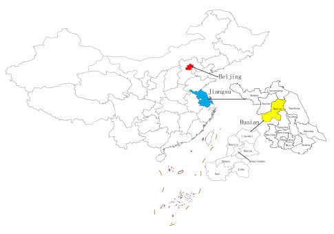
In this paper, we investigate the effects of ambient air pollution (AAP) on the spread of influenza in an AAP-dependent dynamic influenza model. The value of this study lies in two aspects. Mathematically, we establish the threshold dynamics in the term of the basic reproduction number $ \mathcal{R}_0 $: If $ \mathcal{R}_0 < 1 $, the disease will go to extinction, while if $ \mathcal{R}_0 > 1 $, the disease will persist. Epidemiologically, based on the statistical data in Huaian, China, we find that, in order to control the prevalence of influenza, we must increase the vaccination rate, the recovery rate and the depletion rate, and decrease the rate of the vaccine wearing off, the uptake coefficient, the effect coefficient of AAP on transmission rate and the baseline rate. To put it simply, we must change our traveling plan and stay at home to reduce the contact rate or increase the close-contact distance and wear protective masks to reduce the influence of the AAP on the influenza transmission.
Citation: Xiaomeng Wang, Xue Wang, Xinzhu Guan, Yun Xu, Kangwei Xu, Qiang Gao, Rong Cai, Yongli Cai. The impact of ambient air pollution on an influenza model with partial immunity and vaccination[J]. Mathematical Biosciences and Engineering, 2023, 20(6): 10284-10303. doi: 10.3934/mbe.2023451
In this paper, we investigate the effects of ambient air pollution (AAP) on the spread of influenza in an AAP-dependent dynamic influenza model. The value of this study lies in two aspects. Mathematically, we establish the threshold dynamics in the term of the basic reproduction number $ \mathcal{R}_0 $: If $ \mathcal{R}_0 < 1 $, the disease will go to extinction, while if $ \mathcal{R}_0 > 1 $, the disease will persist. Epidemiologically, based on the statistical data in Huaian, China, we find that, in order to control the prevalence of influenza, we must increase the vaccination rate, the recovery rate and the depletion rate, and decrease the rate of the vaccine wearing off, the uptake coefficient, the effect coefficient of AAP on transmission rate and the baseline rate. To put it simply, we must change our traveling plan and stay at home to reduce the contact rate or increase the close-contact distance and wear protective masks to reduce the influence of the AAP on the influenza transmission.

| [1] | World Health Organization, Influenza (seasonal), 2022. Available from: https://www.who.int/news-room/fact-sheets/detail/influenza-(seasonal). |
| [2] | World Health Organization, Ambient (outdoor) air pollution, 2022. Available from: https://www.who.int/news-room/fact-sheets/detail/ambient-(outdoor)-air-quality-and-health. |
| [3] |
N. H. L. Leung, Transmissibility and transmission of respiratory viruses, Nat. Rev. Microbiol., 19 (2021), 528–545. https://doi.org/10.1038/s41579-021-00535-6 doi: 10.1038/s41579-021-00535-6

|
| [4] |
T. C. Hsiao, P. C. Cheng, K. H. Chi, H. Y. Wang, S. Pan, C. Kao, et al., Interactions of chemical components in ambient PM$_{2.5}$ with influenza viruses, J. Hazard. Mater., 423 (2022), 127243. https://doi.org/10.1016/j.jhazmat.2021.127243 doi: 10.1016/j.jhazmat.2021.127243
|
| [5] |
W. Liu, S. Zhao, R. Gong, Y. Zhang, F. Ding, L. Zhang, et al., Interactive effects of meteorological factors and ambient air pollutants on mumps incidences in Ningxia, China between 2015 and 2019, Front. Environ. Sci., 10 (2022), 937450. https://doi.org/10.3389/fenvs.2022.937450 doi: 10.3389/fenvs.2022.937450
|
| [6] |
Y. Cai, J. Li, Y. Kang, K. Wang, W. Wang, The fluctuation impact of human mobility on the influenza transmission, J. Franklin Inst., 357 (2020), 8899–8924. https://doi.org/10.1016/j.jfranklin.2020.07.002 doi: 10.1016/j.jfranklin.2020.07.002
|
| [7] |
M. B. Ghori, P. A. Naik, J. Zu, Z. Eskandari, M. Naik, Global dynamics and bifurcation analysis of a fractional-order SEIR epidemic model with saturation incidence rate, Math. Methods Appl. Sci., 45 (2022), 3665–3688. https://doi.org/10.1002/mma.8010 doi: 10.1002/mma.8010
|
| [8] |
P. A. Naik, J. Zu, M. Naik, Stability analysis of a fractional-order cancer model with chaotic dynamics, Int. J. Biomath., 14 (2021). https://doi.org/10.1142/S1793524521500467 doi: 10.1142/S1793524521500467
|
| [9] |
Y. Tan, Y. Cai, X. Sun, K. Wang, R. Yao, W. Wang, et al., A stochastic SICA model for HIV/AIDS transmission, Chaos, Solitons Fractals, 165 (2022), 112768. https://doi.org/10.1016/j.chaos.2022.112768 doi: 10.1016/j.chaos.2022.112768
|
| [10] |
A. Ahmad, M. Farman, P. A. Naik, N. Zafar, A. Akgul, M. U. Saleem, Modeling and numerical investigation of fractional-order bovine babesiosis disease, Numer. Methods Partial Differ. Equations, 37 (2021), 1946–1964. https://doi.org/10.1002/num.22632 doi: 10.1002/num.22632
|
| [11] |
X. Guan, F. Yang, Y. Cai, W. Wang, Global stability of an influenza a model with vaccination, Appl. Math. Lett., 134 (2022), 108322. https://doi.org/10.1016/j.aml.2022.108322 doi: 10.1016/j.aml.2022.108322
|
| [12] |
Z. Wu, Y. Cai, Z. Wang, W. Wang, Global stability of a fractional order SIS epidemic model, J. Differ. Equations, 352 (2023), 221–248. https://doi.org/10.1016/j.jde.2022.12.045 doi: 10.1016/j.jde.2022.12.045
|
| [13] |
A. Seah, L. H. Loo, N. Jamali, M. Maiwald, J. Aik, The influence of air quality and meteorological variations on influenza A and B virus infections in a paediatric population in Singapore, Environ. Res., 216 (2023), 114453. https://doi.org/10.1016/j.envres.2022.114453 doi: 10.1016/j.envres.2022.114453
|
| [14] |
J. Yang, Z. Yang, L. Qi, M. Li, D. Liu, X. Liu, et al., Influence of air pollution on influenza-like illness in China: a nationwide time-series analysis, eBioMedicine, 87 (2023), 104421. https://doi.org/10.1016/j.ebiom.2022.104421 doi: 10.1016/j.ebiom.2022.104421
|
| [15] |
Z. Zhang, L. Xi, L. Yang, X. Lian, J. Du, Y. Cui, et al., Impact of air pollutants on influenza-like illness outpatient visits under urbanization process in the sub-center of Beijing, China, Int. J. Hyg. Environ. Health, 247 (2023), 114076. https://doi.org/10.1016/j.ijheh.2022.114076 doi: 10.1016/j.ijheh.2022.114076
|
| [16] |
L. Huang, L. Zhou, J. Chen, K. Chen, Y. Liu, X. Chen, et al., Acute effects of air pollution on influenza-like illness in Nanjing, China: A population-based study, Chemosphere, 147 (2016), 180–187. http://dx.doi.org/10.1016/j.chemosphere.2015.12.082 doi: 10.1016/j.chemosphere.2015.12.082
|
| [17] |
Y. Meng, Y. Lu, H. Xiang, S. Liu, Short-term effects of ambient air pollution on the incidence of influenza in Wuhan, China: A time-series analysis-sciencedirect, Environ. Res., 192 (2021), 110327. https://doi.org/10.1016/j.envres.2020.110327 doi: 10.1016/j.envres.2020.110327
|
| [18] |
X. Wang, Z. Xu, H. Su, H. Ho, Y. Song, H. Zheng, et al., Ambient particulate matter (PM$_1$, PM$_{2.5}$, PM$_10$) and childhood pneumonia: the smaller particle, the greater short-term impact, Sci. Total Environ., 772 (2021), 145509. https://doi.org/10.1016/j.scitotenv.2021.145509 doi: 10.1016/j.scitotenv.2021.145509
|
| [19] |
X. Zhang, Y. Zhao, A. U. Neumann, Partial immunity and vaccination for influenza, J. Comput. Biol., 17 (2010), 1689–1696. https://doi.org/10.1089/cmb.2009.0003 doi: 10.1089/cmb.2009.0003
|
| [20] |
Q. Huang, L. Parshotam, H. Wang, C. Bampfylde, M. A. Lewis, A model for the impact of contaminants on fish population dynamics, J. Theor. Biol., 334 (2013), 71–79. https://doi.org/10.1016/j.jtbi.2013.05.018 doi: 10.1016/j.jtbi.2013.05.018
|
| [21] |
Q. Huang, H. Wang, M. A. Lewis, The impact of environmental toxins on predator-prey dynamics, J. Theor. Biol., 378 (2015), 12–30. https://doi.org/10.1016/j.jtbi.2015.04.019 doi: 10.1016/j.jtbi.2015.04.019
|
| [22] |
S. Saha, G. P. Samanta, Dynamics of an epidemic model with impact of toxins, Physica A, 527 (2019), 121152. https://doi.org/10.1016/j.physa.2019.121152 doi: 10.1016/j.physa.2019.121152
|
| [23] |
L. Wang, Z. Jin, H. Wang, A switching model for the impact of toxins on the spread of infectious diseases, J. Math. Biol., 77 (2018), 1093–1115. https://doi.org/10.1007/s00285-018-1245-7 doi: 10.1007/s00285-018-1245-7
|
| [24] | J. K. Hale, Theory of Functional Differential Equations, Springer, 1977. https://doi.org/10.1007/978-1-4612-9892-2 |
| [25] |
O. Diekmann, K. Dietz, J. A. P. Heesterbeek, The basic reproduction ratio for sexually transmitted diseases: Ⅰ. theoretical considerations, Math. Biosci., 107 (1991), 325–339. https://doi.org/10.1016/0025-5564(91)90012-8 doi: 10.1016/0025-5564(91)90012-8
|
| [26] |
P. Van den Driessche, J. Watmough, Reproduction numbers and sub-threshold endemic equilibria for compartmental models of disease transmission, Math. Biosci., 180 (2002), 29–48. https://doi.org/10.1016/S0025-5564(02)00108-6 doi: 10.1016/S0025-5564(02)00108-6
|
| [27] |
W. Wang, X. Zhao, Threshold dynamics for compartmental epidemic models in periodic environments, J. Dyn. Differ. Equations, 20 (2008), 699–717. https://doi.org/10.1007/s10884-008-9111-8 doi: 10.1007/s10884-008-9111-8
|
| [28] |
Y. Cai, S. Zhao, Y. Niu, Z. Peng, K. Wang, D. He, et al., Modelling the effects of the contaminated environments on tuberculosis in Jiangsu, China, J. Theor. Biol., 508 (2021), 110453. https://doi.org/10.1016/j.jtbi.2020.110453 doi: 10.1016/j.jtbi.2020.110453
|
| [29] |
Y. Shu, L. Fang, S. J. de Vlas, Y. Gao, J. H. Richardus, W. Cao, Dual seasonal patterns for influenza, China, Emerging Infect. Dis., 16 (2010), 725–726. https://doi.org/10.3201/eid1604.091578 doi: 10.3201/eid1604.091578
|
| [30] | Huaian Commission of Health. Available from: http://wjw.huaian.gov.cn. |
| [31] | China online air quality monitoring and analysis platform. Available from: https://www.aqistudy.cn/historydata/monthdata.php. |
| [32] | Huaian municipal bureau of statistics. Available from: http://tjj.huaian.gov.cn/. |
| [33] |
Q. Cui, Z. Hu, Y. Li, J. Han, Z. Teng, J. Qian, Dynamic variations of the COVID-19 disease at different quarantine strategies in Wuhan and mainland China, J. Infect. Public Health, 13 (2020), 849–855. https://doi.org/10.1016/j.jiph.2020.05.014 doi: 10.1016/j.jiph.2020.05.014
|
| [34] |
Z. Hu, D. Chen, X. Chen, Q. Zhou, Y. Peng, J. Li, et al., CCHZ-DISO: A timely new assessment system for data quality or model performance from Da Dao Zhi Jian, Geophys. Res. Lett., 49 (2022). https://doi.org/10.1029/2022GL100681 doi: 10.1029/2022GL100681
|
| [35] |
Q. Zhou, D. Chen, Z. Hu, X. Chen, Decompositions of Taylor diagram and DISO performance criteria, Int. J. Climatol., 41 (2021), 5726–5732. https://doi.org/10.1002/joc.7149 doi: 10.1002/joc.7149
|
Figures(7) / Tables(5)

Xiaomeng Wang, Xue Wang, Xinzhu Guan, Yun Xu, Kangwei Xu, Qiang Gao, Rong Cai, Yongli Cai. The impact of ambient air pollution on an influenza model with partial immunity and vaccination[J]. Mathematical Biosciences and Engineering, 2023, 20(6): 10284-10303. doi: 10.3934/mbe.2023451


 DownLoad: