A sustainable smart production model for partial outsourcing and reworking

Raj Kumar Bachar; Shaktipada Bhuniya; Ali AlArjani; Santanu Kumar Ghosh; Biswajit Sarkar; Raj Kumar Bachar; Shaktipada Bhuniya; Ali AlArjani; Santanu Kumar Ghosh; Biswajit Sarkar

doi:10.3934/mbe.2023346

Mathematical Biosciences and Engineering

2023, Volume 20, Issue 5: 7981-8009. doi: 10.3934/mbe.2023346

Previous Article Next Article

Research article Special Issues

A sustainable smart production model for partial outsourcing and reworking

1.
Department of Mathematics, Kazi Nazrul University, Asansol 713340, West Bengal, India
2.
Department of Mathematics & Statistics, Banasthali Vidyapith, Rajasthan 304 022, India
3.
Department of Industrial Engineering, College of Engineering, Prince Sattam Bin Abdulaziz University, Al Kharj 11942, Saudi Arabia
4.
Department of Industrial Engineering, Yonsei University, 50 Yonsei-ro, Sinchon-dong, Seodaemun-gu, Seoul 03722, South Korea
5.
Center for Transdisciplinary Research (CFTR), Saveetha Dental College, Saveetha Institute of Medical and Technical Sciences, Saveetha University, 162, Poonamallee High Road, Velappanchavadi, Chennai 600077, Tamil Nadu, India

Academic Editor: Danilo Pelusi

Received: 29 June 2022 Revised: 27 December 2022 Accepted: 05 January 2023 Published: 23 February 2023

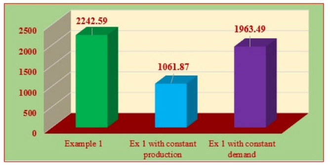
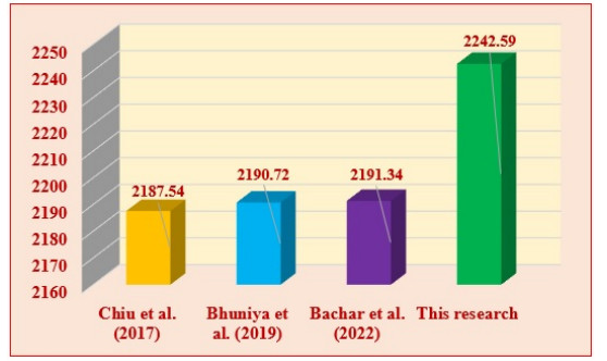
Smart production plays a significant role to maintain good business terms among supply chain players in different situations. Adjustment in production uptime is possible because of the smart production system. The management may need to reduce production uptime to deliver products ontime. But, a decrement in production uptime reduces the projected production quantity. Then, the management uses a limited investment for pursuing possible alternatives to maintain production schedules and the quality of products. This present study develops a mathematical model for a smart production system with partial outsourcing and reworking. The market demand for the product is price dependent. The study aims to maximize the total profit of the production system. Even in a smart production system, defective production rate may be less but unavoidable. Those defective products are repairable. The model is solved by classical optimization. Results show that the application of a variable production rate of the smart production for variable market demand has a higher profit than a traditional production (52.65%) and constant demand (12.45%).
- smart production,
- remanufacturing,
- defective items,
- reworking,
- product outsourcing,
- carbon emissions
Citation: Raj Kumar Bachar, Shaktipada Bhuniya, Ali AlArjani, Santanu Kumar Ghosh, Biswajit Sarkar. A sustainable smart production model for partial outsourcing and reworking[J]. Mathematical Biosciences and Engineering, 2023, 20(5): 7981-8009. doi: 10.3934/mbe.2023346

Related Papers:

Abstract

Smart production plays a significant role to maintain good business terms among supply chain players in different situations. Adjustment in production uptime is possible because of the smart production system. The management may need to reduce production uptime to deliver products ontime. But, a decrement in production uptime reduces the projected production quantity. Then, the management uses a limited investment for pursuing possible alternatives to maintain production schedules and the quality of products. This present study develops a mathematical model for a smart production system with partial outsourcing and reworking. The market demand for the product is price dependent. The study aims to maximize the total profit of the production system. Even in a smart production system, defective production rate may be less but unavoidable. Those defective products are repairable. The model is solved by classical optimization. Results show that the application of a variable production rate of the smart production for variable market demand has a higher profit than a traditional production (52.65%) and constant demand (12.45%).

References

[1]	Y. S. Chiu, C. J. Liu, M. H. Hwang, Optimal batch size considering partial outsourcing plan and rework, Jordan J. Mech. Ind. Eng., 11 (2017), 195–200.
[2]	M. Khouja, A. Mehrez, Economic production lot size model with variable production rate and imperfect quality, J. Oper. Res. Soc., 45 (1994), 1405–1417. https://doi.org/10.1057/jors.1994.217 doi: 10.1057/jors.1994.217
[3]	S. Eiamkanchanalai, A. Banerjee, Production lot sizing with variable production rate and explicit idle capacity cost, Int. J. Prod. Econ., 59 (1999), 251–259. https://doi.org/10.1016/S0925-5273(98)00102-9 doi: 10.1016/S0925-5273(98)00102-9
[4]	B. C. Giri, T. Dohi, Computational aspects of an extended EMQ model with variable production rate, Comput. Oper. Res., 32 (2005), 3143–3161. https://doi.org/10.1016/j.cor.2004.05.004 doi: 10.1016/j.cor.2004.05.004
[5]	C. H. Glock, Batch sizing with controllable production rates, Int. J. Prod. Econ., 48 (2010), 5925–5942. https://doi.org/10.1080/00207540903170906 doi: 10.1080/00207540903170906
[6]	T. Kim, C. H. Glock, Production planning for a two-stage production system with multiple parallel machines and variable production rates, Int. J. Prod. Econ., 196 (2018), 284–292. https://doi.org/10.1016/j.ijpe.2017.11.018 doi: 10.1016/j.ijpe.2017.11.018
[7]	B. Mridha, G. V. Ramana, S. Pareek, B. Sarkar, An efficient sustainable smart approach to biofuel production with emphasizing the environmental and energy aspects, Fuel, 336 (2023), 126896. https://doi.org/10.1016/j.fuel.2022.126896 doi: 10.1016/j.fuel.2022.126896
[8]	A. I. Malik, B. Sarkar, I. Q. Iqbal, M. Ullah, I. Khan, M. B. Ramzan, Coordination supply chain management in flexible production system and service level constraint: A Nash bargaining model, Comp. Indust. Eng., 177 (2023), 109002. https://doi.org/10.1016/j.cie doi: 10.1016/j.cie
[9]	N. Saxena, B. Sarkar, How does the retailing industry decide the best replenishment strategy by utilizing technological support through blockchain?, J. Retail. Consum. Ser., 71 (2023), 103151. https://doi.org/10.1016/j.jretconser.2022.103151 doi: 10.1016/j.jretconser.2022.103151
[10]	W. Shih, Optimal inventory policies when stockouts result from defective products, Int. J. Prod. Res., 18 (1980), 677–686. https://doi.org/10.1080/00207548008919699 doi: 10.1080/00207548008919699
[11]	M. J. Rosenblatt, H. L. Lee, Economic production cycles with imperfect production processes, IIE Trans., 18 (1986), 48–55. https://doi.org/10.1080/07408178608975329 doi: 10.1080/07408178608975329
[12]	T. Boone, R. Ganeshan, Y. Guo, J. K. Ord, The impact of imperfect processes on production run times, Decis. Sci., 31 (2000), 773–787. https://doi.org/10.1111/j.1540-5915.2000.tb00942.x doi: 10.1111/j.1540-5915.2000.tb00942.x
[13]	S. S. Sana, S. K. Goyal, K. Chaudhuri, An imperfect production process in a volume flexible inventory model, Int. J. Prod. Econ., 105 (2007), 548–559. https://doi.org/10.1016/j.ijpe.2006.05.005 doi: 10.1016/j.ijpe.2006.05.005
[14]	T. Chakraborty, B. C. Giri, Lot sizing in a deteriorating production system under inspections, imperfect maintenance and reworks, Oper. Res., 14 (2014), 29–50. https://doi.org/10.1007/s12351-013-0134-5 doi: 10.1007/s12351-013-0134-5
[15]	P. Jawla, S. Singh, Multi-item economic production quantity model for imperfect items with multiple production setups and rework under the effect of preservation technology and learning environment, Int. J. Ind. Eng. Comput., 7 (2016), 703–716. https://doi.org/10.5267/j.ijiec.2016.2.003 doi: 10.5267/j.ijiec.2016.2.003
[16]	B. Sarkar, B. Ganguly, S. Pareek, L. E. Cárdenas-Barrón, A three-echelon green supply chain management for biodegradable products with three transportation modes, Comp. Indust. Eng., 174 (2022), 108727. https://doi.org/10.1016/j.cie.2022.108727 doi: 10.1016/j.cie.2022.108727
[17]	B. Marchi, S. Zanoni, M. Y. Jaber, Economic production quantity model with learning in production, quality, reliability and energy efficiency, Comput. Ind. Eng., 129 (2019), 502–511. https://doi.org/10.1016/j.cie.2019.02.009 doi: 10.1016/j.cie.2019.02.009
[18]	B. Marchi, S. Zanoni, L. E. Zavanella, M. Y. Jaber, Supply chain models with greenhouse gases emissions, energy usage, imperfect process under different coordination decisions, Int. J. Prod. Econ., 211 (2019), 145–153. https://doi.org/10.1016/j.ijpe.2019.01.017 doi: 10.1016/j.ijpe.2019.01.017
[19]	E. Bazan, M. Y. Jaber, S. Zanoni, A review of mathematical inventory models for reverse logistics and the future of its modeling: An environmental perspective, Appl. Math. Modell., 40 (2016), 4151–4178. https://doi.org/10.1016/j.apm.2015.11.027 doi: 10.1016/j.apm.2015.11.027
[20]	S. D. Flapper, R. H. Teunter, Logistic planning of rework with deteriorating work-in-process, Int. J. Prod. Econ., 88 (2004), 51–59. https://doi.org/10.1016/S0925-5273(03)00130-0 doi: 10.1016/S0925-5273(03)00130-0
[21]	P. Biswas, B. R. Sarker, Optimal batch quantity models for a lean production system with in-cycle rework and scrap, Int. J. Prod. Res., 46 (2008), 6585–6610. https://doi.org/10.1080/00207540802230330 doi: 10.1080/00207540802230330
[22]	A. A. Taleizadeh, H. M. Wee, S. J. Sadjadi, Multi-product production quantity model with repair failure and partial backordering, Comput. Ind. Eng., 59 (2010), 45–54. https://doi.org/10.1016/j.cie.2010.02.015 doi: 10.1016/j.cie.2010.02.015
[23]	A. Khanna, A. Kishore, C. Jaggi, Strategic production modeling for defective items with imperfect inspection process, rework, and sales return under two-level trade credit, Int. J. Ind. Eng. Comput., 8 (2017), 85–118. https://doi.org/10.5267/j.ijiec.2016.7.001 doi: 10.5267/j.ijiec.2016.7.001
[24]	R. K. Bachar, S. Bhuniya, S. K. Ghosh, B. Sarkar, Controllable energy consumption in a sustainable smart manufacturing model considering superior service, flexible demand, and partial outsourcing, Mathematics, 10 (2022), 4517. https://doi.org/10.3390/math10234517 doi: 10.3390/math10234517
[25]	S. V. S. Padiyar, V. Vandana, N. Bhagat, S. R. Singh, B. Sarkar, Joint replenishment strategy for deteriorating multi-item through multi-echelon supply chain model with imperfect production under imprecise and inflationary environment, RAIRO-Oper. Res., 56 (2022), 3071–3096. https://doi.org/10.1051/ro/2022071 doi: 10.1051/ro/2022071
[26]	B. C. Das, B. Das, S. K. Mondal, An integrated production-inventory model with defective item dependent stochastic credit period, Comp. Indust. Eng., 110 (2017), 255–263. https://doi.org/10.1016/j.cie.2017.05.025 doi: 10.1016/j.cie.2017.05.025
[27]	A. Coman, B. Ronen, Production outsourcing: a linear programming model for the theory-of-constraints, Int. J. Prod. Res., 38 (2000), 1631–1639. https://doi.org/10.1080/002075400188762 doi: 10.1080/002075400188762
[28]	S. R. Singh, M. Sarkar, B. Sarkar, Effect of learning and forgetting on inventory model under carbon emission and agile manufacturing, Mathematics, 11 (2023), 368. https://doi.org/10.3390/math11020368 doi: 10.3390/math11020368
[29]	G. J. Hahn, T. Sens, C. Decouttere, N. J. Vandaele, A multi-criteria approach to robust outsourcing decision-making in stochastic manufacturing systems, Comput. Ind. Eng., 98 (2016), 275–288. https://doi.org/10.1016/j.cie.2016.05.032 doi: 10.1016/j.cie.2016.05.032
[30]	S. W. Chiu, Y. Y. Li, V. Chiu, Y. S. Chiu, Satisfy product demand with a quality assured hybrid EMQ-based replenishment system, J. Eng. Res., 7 (2019), 225–237.
[31]	S. Bahrami, R. Ghasemi, A new secure and searchable data outsourcing leveraging a Bucket-Chain index tree. J. Inform. Secur. App., 67 (2022), 103206. https://doi.org/10.1016/j.jisa.2022.103206 doi: 10.1016/j.jisa.2022.103206
[32]	S. Kar, K. Basu, B. Sarkar, Advertisement policy for dual-channel within emissions-controlled flexible production system, J. Retail. Consum. Serv., 71 (2023), 103077. https://doi.org/10.1016/j.jretconser.2022.103077 doi: 10.1016/j.jretconser.2022.103077
[33]	R. K. Bachar, S. Bhuniya, S. K. Ghosh, B. Sarkar, Sustainable green production model considering variable demand, partial outsourcing, and rework, AIMS Environ. Sci., 9 (2022), 325–353. https://doi.org/10.3934/environsci.2022022 doi: 10.3934/environsci.2022022
[34]	P. L. Abad, C. K. Jaggi, A joint approach for setting unit price and the length of the credit period for a seller when end demand is price sensitive, Int. J. Prod. Econ., 83 (2003), 115–122. https://doi.org/10.1016/S0925-5273(02)00142-1 doi: 10.1016/S0925-5273(02)00142-1
[35]	B. Pal, S. S. Sana, K. Chaudhuri, Two‐echelon manufacturer–retailer supply chain strategies with price, quality, and promotional effort sensitive demand, Int. Tran. Oper. Res., 22 (2015), 1071–1095. https://doi.org/10.1111/itor.12131 doi: 10.1111/itor.12131
[36]	A. Bhunia, A. Shaikh, A deterministic inventory model for deteriorating items with selling price dependent demand and three-parameter Weibull distributed deterioration, Int. J. Ind. Eng. Comput., 5 (2014), 497–510. https://doi.org/10.5267/j.ijiec.2014.2.002 doi: 10.5267/j.ijiec.2014.2.002
[37]	H. K. Alfares, A. M. Ghaithan, Inventory and pricing model with price-dependent demand, time-varying holding cost, and quantity discounts, Comput. Ind. Eng., 94 (2016), 170–177. https://doi.org/10.1016/j.cie.2016.02.009 doi: 10.1016/j.cie.2016.02.009
[38]	B. Sarkar, B. K. Dey, M. Sarkar, S. J. Kim, A smart production system with an autonomation technology and dual channel retailing, Comput. Ind. Eng., 173 (2022), 108607. https://doi.org/10.1016/j.cie.2022.108607 doi: 10.1016/j.cie.2022.108607
[39]	S. Bhuniya, B. Sarkar, S. Pareek, Multi-product production system with the reduced failure rate and the optimum energy consumption under variable demand, Mathematics, 7 (2019), 465. https://doi.org/10.3390/math7050465 doi: 10.3390/math7050465
[40]	H. Hosseini-Nasab, S. Nasrollahi, M. B. Fakhrzad, M. Honarvar, Transportation cost reduction using cross-docks linking, J. Eng. Res., 11 (2023), 100015. https://doi.org/10.1016/j.jer.2023.100015 doi: 10.1016/j.jer.2023.100015
[41]	U. Chaudhari, A. Bhadoriya, M. Y. Jani, B. Sarkar, A generalized payment policy for deteriorating items when demand depends on price, stock, and advertisement under carbon tax regulations, Mathemat. Comp. Simul., 207 (2023), 556–574. https://doi.org/10.1016/j.matcom.2022.12.015 doi: 10.1016/j.matcom.2022.12.015
[42]	S. K. Hota, S. K. Ghosh, B. Sarkar, A solution to the transportation hazard problem in a supply chain with an unreliable manufacturer, AIMS Environ. Sci., 9 (2022), 354–380. https://doi.org/10.3934/environsci.2022023 doi: 10.3934/environsci.2022023

Reader Comments

your name:*

Email:*
© 2023 the Author(s), licensee AIMS Press. This is an open access article distributed under the terms of the Creative Commons Attribution License (http://creativecommons.org/licenses/by/4.0)