A discrete mixed distribution: Statistical and reliability properties with applications to model COVID-19 data in various countries

Mohamed S. Eliwa; Buthaynah T. Alhumaidan; Raghad N. Alqefari; Mohamed S. Eliwa; Buthaynah T. Alhumaidan; Raghad N. Alqefari

doi:10.3934/mbe.2023340

Mathematical Biosciences and Engineering

2023, Volume 20, Issue 5: 7859-7881. doi: 10.3934/mbe.2023340

Previous Article Next Article

Research article Special Issues

A discrete mixed distribution: Statistical and reliability properties with applications to model COVID-19 data in various countries

1.
Department of Statistics and Operation Research, College of Science, Buraydah 51482, Qassim University, Saudi Arabia
2.
Section of Mathematics, International Telematic University Uninettuno, I-00186 Rome, Italy
3.
Department of Mathematics, Faculty of Science, Mansoura University, Mansoura 35516, Egypt

Academic Editor: Masood Fathi

Received: 29 November 2022 Revised: 05 February 2023 Accepted: 08 February 2023 Published: 22 February 2023

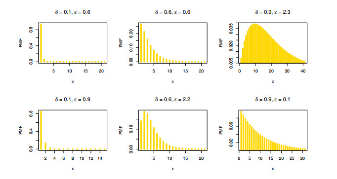
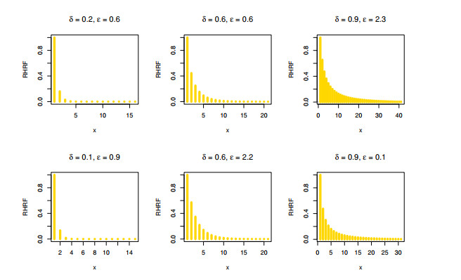
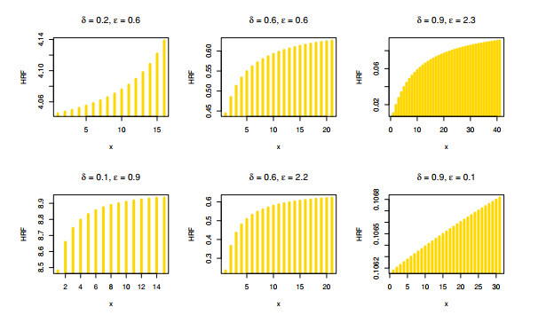
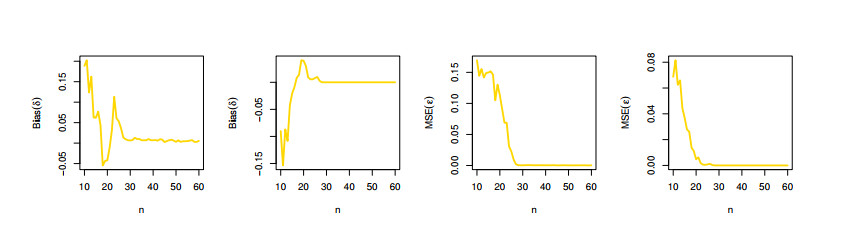
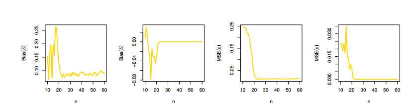
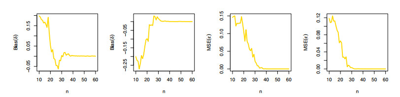
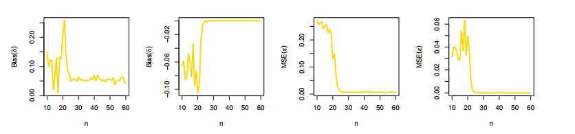
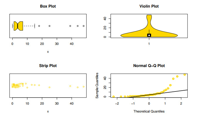
The aim of this paper is to introduce a discrete mixture model from the point of view of reliability and ordered statistics theoretically and practically for modeling extreme and outliers' observations. The base distribution can be expressed as a mixture of gamma and Lindley models. A wide range of the reported model structural properties are investigated. This includes the shape of the probability mass function, hazard rate function, reversed hazard rate function, min-max models, mean residual life, mean past life, moments, order statistics and L-moment statistics. These properties can be formulated as closed forms. It is found that the proposed model can be used effectively to evaluate over- and under-dispersed phenomena. Moreover, it can be applied to analyze asymmetric data under extreme and outliers' notes. To get the competent estimators for modeling observations, the maximum likelihood approach is utilized under conditions of the Newton-Raphson numerical technique. A simulation study is carried out to examine the bias and mean squared error of the estimators. Finally, the flexibility of the discrete mixture model is explained by discussing three COVID-19 data sets.

Keywords:

Citation: Mohamed S. Eliwa, Buthaynah T. Alhumaidan, Raghad N. Alqefari. A discrete mixed distribution: Statistical and reliability properties with applications to model COVID-19 data in various countries[J]. Mathematical Biosciences and Engineering, 2023, 20(5): 7859-7881. doi: 10.3934/mbe.2023340

Related Papers:

[1]	Rashad A. R. Bantan, Zubair Ahmad, Faridoon Khan, Mohammed Elgarhy, Zahra Almaspoor, G. G. Hamedani, Mahmoud El-Morshedy, Ahmed M. Gemeay . Predictive modeling of the COVID-19 data using a new version of the flexible Weibull model and machine learning techniques. Mathematical Biosciences and Engineering, 2023, 20(2): 2847-2873. doi: 10.3934/mbe.2023134
[2]	Mattia Zanella, Chiara Bardelli, Mara Azzi, Silvia Deandrea, Pietro Perotti, Santino Silva, Ennio Cadum, Silvia Figini, Giuseppe Toscani . Social contacts, epidemic spreading and health system. Mathematical modeling and applications to COVID-19 infection. Mathematical Biosciences and Engineering, 2021, 18(4): 3384-3403. doi: 10.3934/mbe.2021169
[3]	Ibrahim Alkhairy . Classical and Bayesian inference for the discrete Poisson Ramos-Louzada distribution with application to COVID-19 data. Mathematical Biosciences and Engineering, 2023, 20(8): 14061-14080. doi: 10.3934/mbe.2023628
[4]	Yinghui Zhou, Zubair Ahmad, Zahra Almaspoor, Faridoon Khan, Elsayed tag-Eldin, Zahoor Iqbal, Mahmoud El-Morshedy . On the implementation of a new version of the Weibull distribution and machine learning approach to model the COVID-19 data. Mathematical Biosciences and Engineering, 2023, 20(1): 337-364. doi: 10.3934/mbe.2023016
[5]	A. Q. Khan, M. Tasneem, M. B. Almatrafi . Discrete-time COVID-19 epidemic model with bifurcation and control. Mathematical Biosciences and Engineering, 2022, 19(2): 1944-1969. doi: 10.3934/mbe.2022092
[6]	Hamdy M. Youssef, Najat A. Alghamdi, Magdy A. Ezzat, Alaa A. El-Bary, Ahmed M. Shawky . A new dynamical modeling SEIR with global analysis applied to the real data of spreading COVID-19 in Saudi Arabia. Mathematical Biosciences and Engineering, 2020, 17(6): 7018-7044. doi: 10.3934/mbe.2020362
[7]	Qinghua Liu, Siyu Yuan, Xinsheng Wang . A SEIARQ model combine with Logistic to predict COVID-19 within small-world networks. Mathematical Biosciences and Engineering, 2023, 20(2): 4006-4017. doi: 10.3934/mbe.2023187
[8]	Ziqiang Cheng, Jin Wang . Modeling epidemic flow with fluid dynamics. Mathematical Biosciences and Engineering, 2022, 19(8): 8334-8360. doi: 10.3934/mbe.2022388
[9]	Salma M. Al-Tuwairqi, Sara K. Al-Harbi . Modeling the effect of random diagnoses on the spread of COVID-19 in Saudi Arabia. Mathematical Biosciences and Engineering, 2022, 19(10): 9792-9824. doi: 10.3934/mbe.2022456
[10]	Enahoro A. Iboi, Oluwaseun Sharomi, Calistus N. Ngonghala, Abba B. Gumel . Mathematical modeling and analysis of COVID-19 pandemic in Nigeria. Mathematical Biosciences and Engineering, 2020, 17(6): 7192-7220. doi: 10.3934/mbe.2020369

Abstract

1. Introduction

The data generated by the daily work environment are more complex in nature at present, and therefore many lifetime models have been listed in the literature to analyze and evaluate these data. Determining which probability distribution should be adopted to make inferences from the data under study is a very important problem in statistics. For these reasons, great efforts have been spent over the years in developing large categories of distributions along with relevant statistical methodologies. See, for instance, El-Gohary et al. ^[1], Saboor et al. ^[2], Jia et al. ^[3], Fernandez ^[4], Alizadeh et al. ^[5], Kumar et al. ^[6], and references cited therein. Nedjar and Zeghdoudi ^[7] proposed a mixture of gamma( $2, \tau$ ) and Lindley( $\varepsilon$ ) (MGL) distributions. The probability density function (PDF) of the MGL distribution can be expressed as

$\begin{equation} g(x;\varepsilon, \tau) = \frac{\tau^{2}}{\varepsilon(1+\tau)}\left( \left[ \tau\varepsilon+\varepsilon-\tau\right] x+1\right) e^{-\tau x} ;\ x > 0, \varepsilon > 0, \tau > 0. \end{equation}$

(1.1)

Unfortunately, Eq (1.1) is not a proper PDF. Messaadia and Zeghdoudi ^[8] corrected the parameter space to be $\varepsilon\geq\frac{\tau }{1+\tau}$ and $\tau > 0$ , and consequently the modified PDF of the MGL model can be written as

$\begin{equation} f(x;\varepsilon, \tau) = \frac{\tau^{2}}{\varepsilon(1+\tau)}\left( \left[ \tau\varepsilon+\varepsilon-\tau\right] x+1\right) e^{-\tau x} ;\ x > 0, \varepsilon\geq\frac{\tau}{1+\tau}, \tau > 0. \end{equation}$

(1.2)

The survival function (SF) corresponding to Eq (1.2) can be formulated as

$\begin{equation} S(x;\varepsilon, \tau) = \frac{(\tau x+1)(\tau\varepsilon+\varepsilon-\tau)+\tau }{\varepsilon(1+\tau)}e^{-\tau x};\ x > 0, \varepsilon\geq\frac{\tau}{1+\tau }, \tau > 0. \end{equation}$

(1.3)

The quantile function (QF) is

$\begin{equation} Q_{X}(u) = \left\{ \begin{array} [c]{l} -\frac{\varepsilon(1+\tau)}{\tau\left[ \varepsilon\left( 1+\tau\right) -\tau\right] }-\frac{1}{\tau}W_{-1}\left( \frac{\varepsilon\left( 1+\tau\right) (u-1)}{\varepsilon\left( 1+\tau\right) -\tau}e^{-\frac {\varepsilon(1+\tau)}{\varepsilon\left( 1+\tau\right) -\tau}}\right) ;\ \varepsilon > \frac{\tau}{1+\tau}\\ \\ \frac{-\ln(1-u)}{\tau} \ \ \ \ \ \ \ \ \ \ \ \ \ \ \ \ \ \ \ \ \ \ \ \ \ \ \ \ \ \ \ \ \ \ \ \ \ \ \ \ \ \ \ \ \ \ \ \ \ ;\ \ \ \varepsilon = \frac{\tau}{1+\tau}, \end{array} \right. \end{equation}$

(1.4)

where $W_{-1}\$ denotes the negative branch of the Lambert $W$ function, and $\frac{-\ln(1-u)}{\tau}$ is the QF of the exponential model. Sometimes, survival trials produce data that are discrete in nature either because of the limitations of the measuring instruments or their inherent characteristics. The study and analysis of counting data plays an important role in many fields of applied sciences, such as economics, engineering, marketing, medicine, and insurance. Counting datasets are often modeled utilizing the Poisson model. However, the Poisson model cannot handle hyper-scattered datasets. Therefore, it is reasonable to model such cases via an appropriate discrete distribution. Discretization of a continuous distribution can be created by using several methods. The most widely utilized technique is the survival discretization approach. For a given continuous random variable $X$ with SF $S(x; \xi ) = \Pr(X > x)$ , we can obtain the discretized version as

$\begin{equation} \Pr(X = x) = S(x;\xi )-S(x+1;\xi );\ x = 0, 1, 2, 3, .... \end{equation}$

(1.5)

For more details, Roy ^[9]. This technique has received a lot of attention in recent years. See, for instance, Gómez-Déniz and Calderín-Ojeda ^[10], Bebbington et al. ^[11], Nekoukhou et al. ^[12], Alamatsaz et al. ^[13], El-Morshedy et al. ^[14], Gillariose et al. ^[15], Singh et al. ^[16,17], Eliwa and El-Morshedy ^[18], Altun et al. ^[19] and references cited therein. In this paper, a discrete distribution MGL (DsMGL) will be discussed from the point of view of reliability and ordered statistics theoretically and practically to analyze extreme and outliers' notes. This is because in El-Morshedy et al. ^[20], simple statistical characteristics and a regression model were presented only in a small whole sample (outliers were not included). Further, the previous paper ignored the reliability, order statistics, and L-moments measures which can be applied in the fields of biomedicine and engineering. Given the importance of reliability and structured statistical measures, the authors sought to discuss neglected characteristics as well as model extreme and outliers' observations. Thus, the motives for this study can be summarized as follows: to formulate statistical characteristics as closed forms; to model dispersed-positively-skewed real data under extreme and outliers' observations; to provide a consistently better fit than other discrete models known in the current statistical literature, especially over-dispersed models; and to prove that the proposed model can be applied to discuss zero-inflated observations.

The article is organized as follows. In Section 2, the DsMGL distribution is proposed. Various properties are derived in Sections 3 and 4. In Section 5, the DsMGL parameters are estimated by utilizing the maximum likelihood approach. Simulation study is discussed in Section 6. In Section 7, three real data sets are analyzed. Finally, some conclusions and future work are listed in Section 8.

2. Discrete analogue of MGL distribution

Recall Eq (1.3), and the SF of the DsMGL distribution can be expressed as

$\begin{equation} S(x;\varepsilon, \delta) = \frac{(1-\ln\delta^{x+1})(\varepsilon-\varepsilon \ln\delta+\ln\delta)-\ln\delta}{\varepsilon(1-\ln\delta)}\delta^{x+1};\ x\in \mathbb{N} _{0}, \end{equation}$

(2.1)

where $\varepsilon\geq\frac{-\ln\delta}{1-\ln\delta}$ , $0 < e^{-\tau} = \delta < 1,$ and $\mathbb{N} _{0} = \left\{ 0, 1, 2, 3, ...\right\}$ . The corresponding PMF to Eq (2.1) can be introduced as

$\begin{equation} P_{x}(x;\varepsilon, \delta) = \frac{\delta^{x}}{1-\ln\delta}\left\{ 1-\delta-\ln\delta\left[ 1+x-\delta(x+2)\right] +(1-\frac{1}{\varepsilon })(\ln\delta)^{2}\left[ x-\delta(x+1)\right] \right\} ;\ x\in \mathbb{N} _{0}. \end{equation}$

(2.2)

The CDF can be reported as

$\begin{equation} F(x;\varepsilon, \delta) = 1-\frac{(1-\ln\delta^{x+1})(\varepsilon-\varepsilon \ln\delta+\ln\delta)-\ln\delta}{\varepsilon(1-\ln\delta)}\delta^{x+1};\ x\in \mathbb{N} _{0}. \end{equation}$

(2.3)

shows the PMF of the DsMGL model based on various values of the parameters $\varepsilon$ and $\delta$ .

Figure 1. The PMF for the DsMGL distribution.

DownLoad: Full-Size Img PowerPoint

As can be noted, the PMF can take unimodal or decreasing form. Moreover, it can be used as a statistical approach to model zero-inflated observations under positive skew.

3. Reliability analytics

In reliability theory, the forward iteration "remaining" time and the past time are two very important measurements in the theory of renewal processes. Consider, for example, the lifetime of a wireless link when a new packet arrives in wireless networks. Reliability studies model the remaining life of a component. If something has survived that far, how long can it be expected to survive? This is the question answered by mean residual life (MRL). In the discrete setting, the MRL, say $\Theta_{i}$ , is defined as

$\begin{equation} \Theta_{i} = \mathbf{E}\left( T-i|T\geq i\right) = \frac{1}{1-F(i-1;\varepsilon , \delta)}\sum\limits_{j = i+1}^{q}\left[ 1-F(j-1;\varepsilon, \delta)\right] ;\ \ i\in \mathbb{N} _{0}, \end{equation}$

(3.1)

where $\mathbb{N} _{0} = \left\{ 0, 1, 2, 3, ..., q\right\}$ for $0 < q < \infty$ . Thus, for the DsMGL model, the MRL is given as

$\begin{equation} \Theta_{i} = -\delta\frac{2(\varepsilon-1)(\delta i-i-1)\ln\delta-\varepsilon (\delta(i+1)-i-2)\ln\delta+\varepsilon(\delta-1)}{(\delta-1)^{2}\left\{ (1-i\ln\delta)(\varepsilon-\varepsilon\ln\delta+\ln\delta)-\ln\delta\right\} };\ \ i\in \mathbb{N} _{0}. \end{equation}$

(3.2)

Furthermore, in the discrete setting, the mean past life (MPL), say $\Theta_{i}^{\ast}$ , is defined as

$\begin{equation} \Theta_{i}^{\ast} = \mathbf{E}\left( i-T|T < i\right) = \frac{1} {F(i-1;\varepsilon, \delta)}\sum\limits_{m = 1}^{i}F(m-1;\varepsilon, \delta);\ \ i\in \mathbb{N} _{0}-\{0\}. \end{equation}$

(3.3)

So, the MPL for the DsMGL model can be represented as

$\begin{align} \Theta_{i}^{\ast} & = \frac{i\varepsilon\delta^{i+2}\ln\delta-i\varepsilon \delta^{i+1}\ln\delta+i\varepsilon\delta^{2}(\ln\delta-1)-2i\delta^{i+2} \ln\delta+2(i+1)\delta^{i+1}\ln\delta-\varepsilon\delta^{i+2}(\ln\delta -1)}{(2i\varepsilon\delta^{i}\ln\delta-2i\delta^{i}\ln\delta-\varepsilon \delta^{i}\ln\delta+\varepsilon\delta^{i}+\varepsilon\ln\delta-\varepsilon )(\delta-1)^{2}}\\ & +\frac{\varepsilon\delta^{2}(\ln\delta-1)-2\delta\ln\delta+(1-2\delta )i\varepsilon\ln\delta+2i\varepsilon\delta-\varepsilon\delta^{i+1} +\varepsilon\delta-i\varepsilon}{(2i\varepsilon\delta^{i}\ln\delta -2i\delta^{i}\ln\delta-\varepsilon\delta^{i}\ln\delta+\varepsilon\delta ^{i}+\varepsilon\ln\delta-\varepsilon)(\delta-1)^{2}}. \end{align}$

(3.4)

For $i\in \mathbb{N} _{0},$ we get $\Theta_{i}^{\ast}\leq i$ . The CDF of the DsMGL model can be recovered by the MPL as

$\begin{equation} F(k;\varepsilon, \delta) = F(0;\varepsilon, \delta) { \prod\limits_{i = 1}^{k}} \left[ \frac{\Theta_{i}^{\ast}}{\Theta_{i+1}^{\ast}-1}\right] ;\ k\in \mathbb{N} _{0}-\{0\}, \end{equation}$

(3.5)

where $F(0;\varepsilon, \delta) = \left({ \prod\limits_{i = 1}^{q}} \left[\frac{\Theta_{i}^{\ast}}{\Theta_{i+1}^{\ast}-1}\right] \right) ^{-1}$ and $0 < q < \infty$ . Thus, the mean of the DsMGL model can be expressed as

$\begin{equation} \text{Mean} = i-\Theta_{i}^{\ast}F(i-1;\varepsilon, \delta)+\Theta_{i}\left[ 1-F(i-1;\varepsilon, \delta)\right] ;\ i\in \mathbb{N} _{0}-\{0\}. \end{equation}$

(3.6)

The reversed hazard rate function (RHRF) can be expressed as a function in MPL as

$\begin{equation} r(i;\varepsilon, \delta) = \frac{1-\Theta_{i+1}^{\ast}+\Theta_{i}^{\ast}} {\Theta_{i}^{\ast}};\ i\in \mathbb{N} _{0}-\{0\}. \end{equation}$

(3.7)

Further, the RHRF can be proposed as

$\begin{equation} r(x;\varepsilon, \delta) = \frac{1-\delta-\ln\delta\left[ 1+x-\delta (x+2)\right] +(1-\frac{1}{\varepsilon})(\ln\delta)^{2}\left[ x-\delta (x+1)\right] }{\varepsilon(1-\ln\delta)-\left[ (1-\ln\delta^{x+1} )(\varepsilon-\varepsilon\ln\delta+\ln\delta)-\ln\delta\right] \delta^{x+1} }\varepsilon\delta^{x};\ \ x\in \mathbb{N} _{0}. \end{equation}$

(3.8)

Figure 2 shows the RHRF plots for different values of the DsMGL parameters.

Figure 2. The RHRF for the DsMGL model.

DownLoad: Full-Size Img PowerPoint

Suppose $W$ and $H$ are two independent DsMGL random variables (RVs) with parameters $(\varepsilon_{1}, \delta_{1})$ and $(\varepsilon_{2}, \delta_{2})$ , respectively. Then, the RHRF of $T = \min(W, H)$ and $L = \max(W, H)$ can be formulated as

$\begin{equation} r_{T}(x;\mathbf{\Lambda}) = 1-\frac{1-\left\{ \frac{(1-\ln\delta_{1} ^{x})(\varepsilon_{1}-\varepsilon_{1}\ln\delta_{1}+\ln\delta_{1})-\ln \delta_{1}}{\varepsilon_{1}(1-\ln\delta_{1})}\delta_{1}^{x}\right\} \left\{ \frac{(1-\ln\delta_{2}^{x})(\varepsilon_{2}-\varepsilon_{2}\ln\delta_{2} +\ln\delta_{2})-\ln\delta_{2}}{\varepsilon_{2}(1-\ln\delta_{2})}\delta_{2} ^{x}\right\} }{1-\left\{ \frac{(1-\ln\delta_{1}^{x+1})(\varepsilon _{1}-\varepsilon_{1}\ln\delta_{1}+\ln\delta_{1})-\ln\delta_{1}}{\varepsilon _{1}(1-\ln\delta_{1})}\delta_{1}^{x+1}\right\} \left\{ \frac{(1-\ln \delta_{2}^{x+1})(\varepsilon_{2}-\varepsilon_{2}\ln\delta_{2}+\ln\delta _{2})-\ln\delta_{2}}{\varepsilon_{2}(1-\ln\delta_{2})}\delta_{2} ^{x+1}\right\} }, \end{equation}$

(3.9)

and

$\begin{align} r_{L}(x;\mathbf{\Lambda}) & = \frac{1-\delta_{1}-\ln\delta_{1}\left[ 1+x-\delta_{1}(x+2)\right] +(1-\frac{1}{\varepsilon_{1}})(\ln\delta_{1} )^{2}\left[ x-\delta_{1}(x+1)\right] }{\varepsilon_{1}(1-\ln\delta _{1})-\left[ (1-\ln\delta_{1}^{x+1})(\varepsilon_{1}-\varepsilon_{1}\ln \delta_{1}+\ln\delta_{1})-\ln\delta_{1}\right] \delta_{1}^{x+1}} \varepsilon_{1}\delta_{1}^{x}\\ & +\frac{1-\delta_{2}-\ln\delta_{2}\left[ 1+x-\delta_{2}(x+2)\right] +(1-\frac{1}{\varepsilon_{2}})(\ln\delta_{2})^{2}\left[ x-\delta _{2}(x+1)\right] }{\varepsilon_{2}(1-\ln\delta_{2})-\left[ (1-\ln\delta _{2}^{x+1})(\varepsilon_{2}-\varepsilon_{2}\ln\delta_{2}+\ln\delta_{2} )-\ln\delta_{2}\right] \delta_{2}^{x+1}}\varepsilon_{2}\delta_{2} ^{x}\\ & -\frac{1-\delta_{1}-\ln\delta_{1}\left[ 1+x-\delta_{1}(x+2)\right] +(1-\frac{1}{\varepsilon_{1}})(\ln\delta_{1})^{2}\left[ x-\delta _{1}(x+1)\right] }{\varepsilon_{1}(1-\ln\delta_{1})-\left[ (1-\ln\delta _{1}^{x+1})(\varepsilon_{1}-\varepsilon_{1}\ln\delta_{1}+\ln\delta_{1} )-\ln\delta_{1}\right] \delta_{1}^{x+1}}\varepsilon_{1}\delta_{1} ^{x}\\ & \times\frac{1-\delta_{2}-\ln\delta_{2}\left[ 1+x-\delta_{2}(x+2)\right] +(1-\frac{1}{\varepsilon_{2}})(\ln\delta_{2})^{2}\left[ x-\delta _{2}(x+1)\right] }{\varepsilon_{2}(1-\ln\delta_{2})-\left[ (1-\ln\delta _{2}^{x+1})(\varepsilon_{2}-\varepsilon_{2}\ln\delta_{2}+\ln\delta_{2} )-\ln\delta_{2}\right] \delta_{2}^{x+1}}\varepsilon_{2}\delta_{2}^{x}. \end{align}$

(3.10)

Since the RHRFs of the two RVs $W$ and $H$ are decreasing, then the RHRFs of $T = \min(W, H)$ and $L = \max(W, H)$ are also decreasing. Another important measure in survival analysis theory is called the hazard rate function (HRF). If $X$ is a DsMGL random variable, then the HRF can be expressed as

$\begin{equation} h(x;\varepsilon, \delta) = 1-\frac{\left[ (1-\ln\delta^{x+1})(\varepsilon -\varepsilon\ln\delta+\ln\delta)-\ln\delta\right] \delta}{(1-\ln\delta ^{x})(\varepsilon-\varepsilon\ln\delta+\ln\delta)-\ln\delta};\ \ x\in \mathbb{N} _{0}, \end{equation}$

(3.11)

where $h(x; \varepsilon, \delta) = \frac{P_{x}(x; \varepsilon, \delta)} {S(x-1;\varepsilon, \delta)}$ . Figure 3 shows the HRF plots for different values of the DsMGL parameters. It should be noted that the new paradigm can be used to discuss any phenomena of an increasing unilateral form.

Figure 3. The HRF for the DsMGL distribution.

DownLoad: Full-Size Img PowerPoint

Suppose $W$ and $H$ are two independent RVs with parameters DsMGL $(\varepsilon _{1}, \delta_{2})$ and DsMGL $(\varepsilon_{2}, \delta_{2})$ , respectively. Then, the HRF of $T = \min(W, H)$ can be formulated as

$\begin{align*} h_{T}(x;\mathbf{\Lambda}) & = \frac{\mathbf{\Pr}(\text{min}(W, H) = x)} {\mathbf{\Pr}(\text{min}(W, H)\geq x)}\\ & = \frac{\mathbf{\Pr}(\text{min}(W, H)\geq x)-\Pr(\text{min}(W, H)\geq x+1)}{\mathbf{\Pr}(\text{min}(W, H)\geq x)}\\ & = \frac{\mathbf{\Pr}(W\geq x)\mathbf{\Pr}(H\geq x)-\mathbf{\Pr}(W\geq x+1)\mathbf{\Pr}(H\geq x+1)}{\mathbf{\Pr}(W\geq x)\mathbf{\Pr}(V\geq x)}\\ & = \frac{\mathbf{\Pr}(W\geq x)\mathbf{\Pr}(H = x)+\mathbf{\Pr}(W = x)\mathbf{\Pr }(H\geq x)-\mathbf{\Pr}(W = x)\mathbf{\Pr}(H = x)}{\mathbf{\Pr}(W\geq x)\mathbf{\Pr}(H\geq x)}, \end{align*}$

where $\mathbf{\Lambda} = (\varepsilon_{1}, \varepsilon_{2}, \delta_{1}, \delta _{2}).$ Then,

$\begin{align} h_{T}(x;\mathbf{\Lambda}) & = \left\{ 1-\frac{\left[ (1-\ln\delta_{1} ^{x+1})(\varepsilon_{1}-\varepsilon_{1}\ln\delta_{1}+\ln\delta_{1})-\ln \delta_{1}\right] \delta_{1}}{(1-\ln\delta_{1}^{x})(\varepsilon _{1}-\varepsilon_{1}\ln\delta_{1}+\ln\delta_{1})-\ln\delta_{1}}\right\} \\ & +\left\{ 1-\frac{\left[ (1-\ln\delta_{2}^{x+1})(\varepsilon_{2} -\varepsilon_{2}\ln\delta_{2}+\ln\delta_{2})-\ln\delta_{2}\right] \delta_{2} }{(1-\ln\delta_{2}^{x})(\varepsilon_{2}-\varepsilon_{2}\ln\delta_{2}+\ln \delta_{2})-\ln\delta_{2}}\right\} \\ & -\left\{ 1-\frac{\left[ (1-\ln\delta_{1}^{x+1})(\varepsilon_{1} -\varepsilon_{1}\ln\delta_{1}+\ln\delta_{1})-\ln\delta_{1}\right] \delta_{1} }{(1-\ln\delta_{1}^{x})(\varepsilon_{1}-\varepsilon_{1}\ln\delta_{1}+\ln \delta_{1})-\ln\delta_{1}}\right\} \\ & \times\left\{ 1-\frac{\left[ (1-\ln\delta_{2}^{x+1})(\varepsilon _{2}-\varepsilon_{2}\ln\delta_{2}+\ln\delta_{2})-\ln\delta_{2}\right] \delta_{2}}{(1-\ln\delta_{2}^{x})(\varepsilon_{2}-\varepsilon_{2}\ln\delta _{2}+\ln\delta_{2})-\ln\delta_{2}}\right\} . \end{align}$

(3.12)

Since the HRFs of the two RVs $W$ and $H$ are increasing, the HRF of $T = \min(W, H)$ is also increasing. Similarly, the HRF of $L = \max(W, H)$ can be expressed as

$\begin{equation} h_{L}(x;\mathbf{\Lambda}) = 1-\frac{1-\left\{ 1-\frac{(1-\ln\delta_{1} ^{x+1})(\varepsilon_{1}-\varepsilon_{1}\ln\delta_{1}+\ln\delta_{1})-\ln \delta_{1}}{\varepsilon_{1}(1-\ln\delta_{1})}\delta_{1}^{x+1}\right\} \left\{ 1-\frac{(1-\ln\delta_{2}^{x+1})(\varepsilon_{2}-\varepsilon_{2} \ln\delta_{2}+\ln\delta_{2})-\ln\delta_{2}}{\varepsilon_{2}(1-\ln\delta_{2} )}\delta_{2}^{x+1}\right\} }{1-\left\{ 1-\frac{(1-\ln\delta_{1} ^{x})(\varepsilon_{1}-\varepsilon_{1}\ln\delta_{1}+\ln\delta_{1})-\ln \delta_{1}}{\varepsilon_{1}(1-\ln\delta_{1})}\delta_{1}^{x}\right\} \left\{ 1-\frac{(1-\ln\delta_{2}^{x})(\varepsilon_{2}-\varepsilon_{2}\ln\delta_{2} +\ln\delta_{2})-\ln\delta_{2}}{\varepsilon_{2}(1-\ln\delta_{2})}\delta_{2} ^{x}\right\} }. \end{equation}$

(3.13)

4. Some distributive properties

4.1. The DsMGL distribution for order statistics: PMF and moments

Assume $X_{1:l}, X_{2:l}, ..., X_{l:l}$ are the corresponding order statistics (OS) of the random sample (RS) $X_{1}, X_{2}, ..., \ X_{l}$ from the DsMGL model. Then, the CDF of the $i$ th OS is given as

$\begin{align} F_{i:l}(x;\varepsilon, \delta) & = \sum\limits_{b = i}^{l}\left( \begin{array} [c]{c} l\\ b \end{array} \right) \left[ F_{i}(x;\varepsilon, \delta\right] ^{b}\left[ 1-F_{i} (x;\varepsilon, \delta)\right] ^{l-b}\\ & = \sum\limits_{b = i}^{l}\sum\limits_{j = 0}^{l-b}\vartheta_{(m)}^{(l, b)}F_{i}(x;\varepsilon , \delta, b+j), \end{align}$

(4.1)

where $\vartheta_{(m)}^{(l, b)} = (-1)^{j}\left(\begin{array} [c]{c} l\\ b \end{array} \right) \left(\begin{array} [c]{c} l-b\\ j \end{array} \right)$ . The corresponding PMF to Eq (4.1) can be listed as

$\begin{align} f_{i:l}(x;\varepsilon, \delta) & = F_{i:l}(x;\varepsilon, \delta)-F_{i:l} (x-1;\varepsilon, \delta)\\ & = \sum\limits_{b = i}^{l}\sum\limits_{j = 0}^{l-b}\vartheta_{(m)}^{(l, b)}f_{i}(x;\varepsilon , \delta, b+j), \end{align}$

(4.2)

where $f_{i}(x; \varepsilon, \delta, b+j)$ represents the PMF of the exponentiated DsMGL distribution with power parameter $b+j.$ So, the $vth$ moments of $X_{i:l}$ can be written as

$\begin{equation} E(X_{i:l}^{v}) = \sum\limits_{x = 0}^{\infty}\sum\limits_{b = i}^{l}\sum\limits_{j = 0}^{l-b} \vartheta_{(m)}^{(l, b)}x^{v}f_{i}(x;\varepsilon, \delta, b+j). \end{equation}$

(4.3)

Hosking ^[21] has defined the L-moment (L-MT) to show the descriptive statistics for the probability model. The L-MT of the DsMGL can be formulated as

$\begin{equation} \Upsilon o = \frac{1}{o}\sum\limits_{c = 0}^{o-1}(-1)^{c}\left( \begin{array} [c]{c} o-1\\ c \end{array} \right) E\left( X_{o-c:o}\right) . \end{equation}$

(4.4)

Using Eq (4.4), L-MT of mean $= \Upsilon_{1}$ , L-MT coefficient of variation $= \frac{\Upsilon_{2}}{\Upsilon_{1}}$ , L-MT coefficient of skewness $= \frac{\Upsilon_{3}}{\Upsilon_{2}},$ and L-MT coefficient of kurtosis $= \frac{\Upsilon_{4}}{\Upsilon_{2}}$ .

4.2. The original moments for data behavior scan

The shape of any probability model can be described by its different moments. Based on the first four moments, the mean " $E(X)$ ", variance " $Var(X)$ ", index of dispersion " $D(X)$ ", skewness " $Sk(X)$ ", and kurtosis " $Ku(X)$ " can be derived. Let $X$ be a DsMGL random variable. Then, the probability generating function (PGF), say $\Upsilon(z)$ , can be formulated as

$\begin{align} \Upsilon(z) & = \sum\limits_{x = 0}^{\infty}z^{x}P_{x}(x;\varepsilon, \delta)\\ & = \frac{1}{1-\ln\delta}\sum\limits_{x = 0}^{\infty}\left\{ 1-\delta-\ln\delta\left[ 1+x-\delta(x+2)\right] +(1-\frac{1}{\varepsilon})(\ln\delta)^{2}\left[ x-\delta(x+1)\right] \right\} (z\delta)^{x}\\ & = \frac{-2\delta(\varepsilon-1)(z-1)\ln\delta+\varepsilon\left( \delta ^{2}z-2\delta+1\right) \ln\delta-\varepsilon(\delta-1)(\delta z-1)} {\varepsilon(\ln\delta-1)(\delta z-1)^{2}}, \end{align}$

(4.5)

where the power series converges absolutely at least for all complex numbers $z$ with $|z|\leq1$ . Equation (4.5) can be derived utilizing the Maple software program. Thus, the first four moments of the DsMGL model can be listed as

$\begin{equation} E(X) = -\delta\frac{\left( \varepsilon-1\right) \ln\delta^{2}+\varepsilon (\delta-2)\ln\delta-\varepsilon(\delta-1)}{\varepsilon(\ln\delta -1)(\delta-1)^{2}}, \end{equation}$

(4.6)

$\begin{equation} E(X^{2}) = \delta\frac{\left( 3\varepsilon\delta+\varepsilon-3\delta-1\right) \ln\delta^{2}+\varepsilon(\delta^{2}-3\delta-2)\ln\delta-\varepsilon\delta ^{2}+\varepsilon}{\varepsilon(\ln\delta-1)(\delta-1)^{3}}, \end{equation}$

(4.7)

$\begin{equation} E(X^{3}) = -\delta\frac{14\left( \delta^{2}+\frac{10}{7}\delta+\frac{1} {7}\right) \left( \varepsilon-1\right) \ln\delta+\varepsilon(\delta +2)(\delta^{2}-6\delta-1)\ln\delta-\varepsilon(\delta-1)(\delta^{2} +4\delta+1)}{\varepsilon(\ln\delta-1)(\delta-1)^{4}}, \end{equation}$

(4.8)

and

$\begin{align} E(X^{4}) & = \delta\frac{30\left( \delta^{3}+\frac{11}{3}\delta^{2}+\frac {5}{3}\delta+\frac{1}{15}\right) \left( \varepsilon-1\right) \ln \delta+\varepsilon(\delta^{4}-5\delta^{3}-55\delta^{2}-35\delta-2)\ln\delta }{\varepsilon(\ln\delta-1)(\delta-1)^{5}}\\ & -\frac{\delta^{4}+10\delta^{3}-10\delta-1}{(\ln\delta-1)(\delta-1)^{5} }. \end{align}$

(4.9)

According to the previous moments " $E(X^{r}); \ r = 1, 2, 3, 4$ ", the $E(X)$ , $Var(X)$ , $Sk(X)$ , and $Ku(X)$ can be derived in closed forms. Table 1 reports some numerical results for the DsMGL model under different values of the distribution parameters.

Table 1. Some descriptive statistics under

$\delta = 0.05\$ and various values of

$\varepsilon$ .

	$\varepsilon$
Measure	$1.1$	$1.4$	$1.7$	$2.1$	$4.2$	$8.4$
$E(X)$	$0.10548$	$0.12972$	$0.14540$	$0.15934$	$0.18897$	$0.20378$
$Var(X)$	$0.11102$	$0.13466$	$0.14933$	$0.16196$	$0.18750$	$0.19962$
$D(X)$	$1.05252$	$1.03809$	$1.02701$	$1.01641$	$0.99223$	$0.97955$
$Sk(X)$	$3.31652$	$2.93747$	$2.73625$	$2.57885$	$2.29485$	$2.17274$
$Ku(X)$	$14.9956$	$12.2687$	$10.94861$	$9.97976$	$8.37673$	$7.74605$

| Show Table

DownLoad: CSV

The DsMGL is capable of modeling positively skewed and leptokurtic datasets. Further, it is appropriate for modeling under- (over-) dispersed phenomena where $\frac{Var(X)}{|E(X)|} < (>)1$ for some parameter values.

5. Estimation of the DsMGL parameters

In this segment, the maximum likelihood estimates (MLEs) of the model parameters are determined. Let $X_{1}, X_{2}, ..., X_{n}$ be a RS of size $n$ from the DsMGL distribution. The log-likelihood function ( $LL$ ) can be written as

$\begin{equation} LL(x;\varepsilon, \delta) = \ln\delta { \sum\limits_{i = 1}^{n}} x_{i}-n\ln\left( 1-\ln\delta\right) + { \sum\limits_{i = 1}^{n}} \ln\left( 1-\delta-\ln\delta\left[ 1+x_{i}-\delta(x_{i}+2)\right] +(1-\frac{1}{\varepsilon})(\ln\delta)^{2}\left[ x_{i}-\delta(x_{i}+1)\right] \right) . \end{equation}$

(5.1)

The MLEs of the parameters $\varepsilon$ and $\delta$ , say $\widehat{\varepsilon}$ and $\widehat{\delta}$ , are derived by $(\widehat{\varepsilon}, \widehat{\delta})$ $= \$ argmax $_{(\varepsilon, \delta)}\ (L)$ or, in an equivalent approach in our case, $(\widehat{\varepsilon }, \widehat{\delta})$ $= \$ argmax $_{(\varepsilon, \delta)}\ (LL)$ . To provide more practicalities, the normal equations can be formulated as

$\begin{equation} \frac{\partial LL(x;\varepsilon, \delta)}{\partial\varepsilon} = { \sum\limits_{i = 1}^{n}} \frac{\left( \frac{\ln\delta}{\varepsilon}\right) ^{2}\left[ x_{i} -\delta(x_{i}+1)\right] }{1-\delta-\ln\delta\left[ 1+x_{i}-\delta (x_{i}+2)\right] +(1-\frac{1}{\varepsilon})(\ln\delta)^{2}\left[ x_{i}-\delta(x_{i}+1)\right] } \end{equation}$

(5.2)

and

$\begin{align} \frac{\partial LL(x;\varepsilon, \delta)}{\partial\delta} & = \frac{1}{\delta} { \sum\limits_{i = 1}^{n}} x_{i}+\frac{n}{\delta\left( 1-\ln\delta\right) }\\ & + { \sum\limits_{i = 1}^{n}} \frac{\left( x_{i}+2\right) \left( \ln\delta+1\right) -\frac{1+x_{i} }{\delta}-1+\ln\delta\left( 1-\frac{1}{\varepsilon}\right) \left( \frac{2x_{i}-2\delta(x_{i}+1)}{\delta}-(x_{i}+1)\ln\delta\right) } {1-\delta-\ln\delta\left[ 1+x_{i}-\delta(x_{i}+2)\right] +(1-\frac {1}{\varepsilon})(\ln\delta)^{2}\left[ x_{i}-\delta(x_{i}+1)\right] }. \end{align}$

(5.3)

The two previous equations cannot be solved analytically; therefore, a mathematical package such as the R program based on an iterative procedure such as the Newton-Raphson (numerical optimization approach) can be used to obtain the estimators.

6. Simulation: Appreciative behavior of estimators

In this segment, Monte Carlo simulation was performed to prove the efficiency of the DsMGL model utilizing the maximum likelihood approach. The performance of the MLE with respect to sample size $n$ is tested. The evaluation is based on a simulation study:

$1)$ Generate $10000$ samples of size $n =$ $10, 11, 12, ..., 60$ from the DsMGL model based on four cases as follows: case I: $(\delta = 0.1$ and $\varepsilon = 0.9)$ , case II: $(\delta = 0.3\$ and $\varepsilon = 0.9)$ , case III: $(\delta = 0.5\$ and $\varepsilon = 0.9)$ , and case IV: $(\delta = 0.7\$ and $\varepsilon = 0.9)$ .

$2)$ Generate $10000$ samples of size $n =$ $30, 70, 140, 200, 300, 400, 600$ from the DsMGL model based on four cases as follows: case V: $(\delta = 0.5$ and $\varepsilon = 0.4)$ , case VI: $(\delta = 0.5\$ and $\varepsilon = 0.5)$ , case VII: $(\delta = 0.5\$ and $\varepsilon = 1.5)$ , and case VIII: $(\delta = 0.5\$ and $\varepsilon = 2.0)$ .

$3)$ Compute the MLEs for the $10000$ samples, say $\widehat{\varepsilon} _{j}$ and $\widehat{\delta}_{j}$ for $j = 1, 2, 3, ..., 1000$ .

$4)$ Compute the biases, mean-squared errors (MSE), and mean relative errors (MRE).

$5)$ The empirical results are shown in Figures 4–7 and Tables 2 and 3.

Figure 4. The empirical results based on case I.

DownLoad: Full-Size Img PowerPoint

Figure 5. The empirical results based on case II.

DownLoad: Full-Size Img PowerPoint

Figure 6. The empirical results based on case III.

DownLoad: Full-Size Img PowerPoint

Figure 7. The empirical results based on case IV.

DownLoad: Full-Size Img PowerPoint

Table 2. The empirical simulation results for schemes V and VI.

		Scheme V			Scheme VI
Parameter	$n$	Bias	MSE	MRE	Bias	MSE	MRE
$\delta$	$30$	$0.10056591$	$0.09006876$	$0.06336994$	$0.11632194$	$0.08963175$	$0.08223158$
	$70$	$0.09865782$	$0.08830367$	$0.04163261$	$0.10223666$	$0.06202190$	$0.08063179$
	$140$	$0.04369310$	$0.08200239$	$0.04001453$	$0.09220169$	$0.06101429$	$0.07312016$
	$200$	$0.02299658$	$0.07703927$	$0.03192237$	$0.08139327$	$0.04002236$	$0.06350036$
	$300$	$0.02126971$	$0.06005479$	$0.02101206$	$0.08023636$	$0.03237014$	$0.05519738$
	$400$	$0.01733369$	$0.04079031$	$0.00700269$	$0.05193079$	$0.01112539$	$0.04980373$
	$600$	$0.00234104$	$0.00201034$	$0.00023694$	$0.00292733$	$0.00026456$	$0.00015654$
$\varepsilon$	$30$	$0.09369110$	$0.07793171$	$0.06131304$	$0.05969637$	$0.04320158$	$0.05336947$
	$70$	$0.08567341$	$0.07122367$	$0.05510375$	$0.05223691$	$0.03201392$	$0.05102125$
	$140$	$0.07011036$	$0.06379035$	$0.05022693$	$0.04112566$	$0.03036549$	$0.04020024$
	$200$	$0.04105604$	$0.05380086$	$0.04500102$	$0.03233697$	$0.02002137$	$0.03102236$
	$300$	$0.03367101$	$0.04522564$	$0.04103979$	$0.03102973$	$0.01122024$	$0.01909439$
	$400$	$0.02098200$	$0.03474369$	$0.03139064$	$0.01018674$	$0.00889001$	$0.00306970$
	$600$	$0.00523689$	$0.00236844$	$0.00053671$	$0.00235659$	$0.00059458$	$0.00002518$

| Show Table

DownLoad: CSV

Table 3. The empirical simulation results for schemes VII and VIII.

		Scheme VII			Scheme VIII
Parameter	$n$	Bias	MSE	MRE	Bias	MSE	MRE
$\delta$	$30$	$0.025687193$	$0.01466875$	$0.01399737$	$0.06696575$	$0.08763274$	$0.06353187$
	$70$	$0.022658763$	$0.01136219$	$0.10145190$	$0.06132640$	$0.06923671$	$0.06123671$
	$140$	$0.019365811$	$0.00855157$	$0.00500215$	$0.05426598$	$0.05110123$	$0.05922014$
	$200$	$0.015330240$	$0.00431502$	$0.00362307$	$0.05120134$	$0.04320139$	$0.04623665$
	$300$	$0.013695875$	$0.00400236$	$0.00306981$	$0.05026971$	$0.03915618$	$0.04010656$
	$400$	$0.008532179$	$0.00100153$	$0.00168892$	$0.04902790$	$0.03101569$	$0.03410973$
	$600$	$0.001036942$	$0.00010265$	$0.00023296$	$0.00265235$	$0.00021691$	$0.00139237$
$\varepsilon$	$30$	$0.108067988$	$0.01123177$	$0.08307104$	$0.07437669$	$0.07782736$	$0.09069587$
	$70$	$0.103365789$	$0.00998796$	$0.08223676$	$0.06722364$	$0.05220104$	$0.08133658$
	$140$	$0.089445810$	$0.00912348$	$0.07911671$	$0.04749836$	$0.03002336$	$0.06310263$
	$200$	$0.071002158$	$0.00722369$	$0.06600163$	$0.03229659$	$0.01024787$	$0.05154031$
	$300$	$0.053210199$	$0.00426971$	$0.03697274$	$0.03193261$	$0.01010915$	$0.03974904$
	$400$	$0.009571377$	$0.00379104$	$0.00409265$	$0.02410124$	$0.00580048$	$0.02122360$
	$600$	$0.000531041$	$0.00022165$	$0.00023291$	$0.00124304$	$0.00083190$	$0.00212642$

| Show Table

DownLoad: CSV

According to Figures 4–7 and and , the magnitude of bias, MSE, and MRE always decrease to zero as $n$ grows (consistency property). Thus, the MLE approach can be utilized effectively for the parameter's estimation.

7. Data modeling

In this section, we demonstrate the resilience of the DsMGL distribution in modeling COVID-19 data. Fitted models are compared using some criteria, namely, the $-LL$ , Akaike-information-criterion (AIC), modified-AIC (MAIC), Hannan-Quinn-information-criterion (HQIC), Bayesian-information-criterion (BIC), and Kolmogorov-Smirnov (K-S) test with its corresponding P-value. We will compare the flexibility of the DsMGL model with some of the competitive models such as discrete Lindley (DsL), discrete Burr-Hatke (DsBH), new discrete distribution with one parameter (NDsIP) (see, Eliwa and El-Morshedy, 2022), discrete Rayleigh (DsR), discrete Pareto (DsPa), discrete Burr type XII (DsB-XII), and modified negative binomial (NeBi) models.

7.1. Data set I: COVID-19 in Hong Kong

The data is listed in (https://www.worldometers.info/coronavirus/country/china-hong-kong-sar/) and represents the daily new cases in Hong Kong for COVID-19 from Feb. 15, 2020, to Oct. 25, 2020. The initial shape/form of this data is reported in Figure 8 using non-parametric (N-P) methods like strip, box, violin and QQ plots. It is noted that there are extreme and outliers' observations.

Figure 8. The N-P plots for COVID-19 data in Hong Kong.

DownLoad: Full-Size Img PowerPoint

The MLEs with their corresponding standard error (SE), confidence interval (C. I) for the parameter(s) and goodness-of-fit test (G-O-F-T) for COVID-19 data in Hong Kong, are listed in Tables 4 and 5.

Table 4. The MLEs with their corresponding SE and C. I for COVID-19 data in Hong Kong.

	$\varepsilon$			$\delta$
Model	MLE	SE	C. I	MLE	SE	C. I
DsMGL	$0.8887$	$0.0242$	$[0.8390, 0.9361]$	$0.1062$	$0.0373$	$[0.0355, 0.1786]$
DsL	$0.8052$	$0.0200$	$[0.7660, 0.8451]$	$-$	$-$	$-$
NDsIP	$0.9110$	$0.0151$	$[0.8820, 0.9390]$	$-$	$-$	$-$
DsR	$0.9951$	$0.1361$	$[0.7280, 1.000]$	$-$	$-$	$-$
DsB-XII	$0.8173$	$0.0740$	$[0.6722, 0.9622]$	$3.2981$	$1.4272$	$[0.5013, 6.0962]$
DsPa	$0.5592$	$0.0531$	$[0.4515, 0.6603]$	$-$	$-$	$-$
DsBH	$0.9954$	$0.0132$	$[0.9695, 1.000]$	$-$	$-$	$-$
NeBi	$0.9203$	$0.0221$	$[0.8772, 0.9634]$	$0.6859$	$0.1023$	$[0.4854, 0.8864]$

| Show Table

DownLoad: CSV

Table 5. The G-O-F-T for COVID-19 data in Hong Kong.

	Model
Statistic	DsMGL	DsL	NDsIP	DsR	DsB-XII	DsPa	DsBH	NeBi
$\mathbf{-}LL$	$118.951$	$127.120$	$121.353$	$161.193$	$118.992$	$124.333$	$130.953$	$119.237$
AIC	$241.892$	$256.234$	$244.717$	$324.384$	$241.980$	$250.662$	$263.902$	$242.473$
MAIC	$242.233$	$256.343$	$244.824$	$324.493$	$242.325$	$250.777$	$264.014$	$242.816$
BIC	$245.178$	$257.877$	$246.352$	$326.024$	$245.263$	$252.302$	$265.543$	$245.748$
HQIC	$243.065$	$256.825$	$245.295$	$324.963$	$243.157$	$251.254$	$264.484$	$243.638$
K-S	$0.157$	$0.246$	$0.186$	$0.761$	$0.277$	$0.367$	$0.565$	$0.167$
P-value	$0.305$	$0.020$	$0.146$	$\leq0.001$	$0.006$	$\leq0.001$	$\leq0.001$	$0.285$

| Show Table

DownLoad: CSV

The DsMGL model is the best among all the discussed models, because it has the lowest value among $-LL$ , AIC, MAIC, BIC, HQIC and K-S. Moreover, the DsMGL model has the highest P-value among all tested distributions. Figures 9 and 10 show the estimated CDF and P-P plots for all reported models from which the distribution adequacy of the DsMGL model can be noted clearly. Thus, the COVID-19 data in Hong Kong plausibly came from the DsMGL model.

Figure 9. The estimated CDFs for COVID-19 data in Hong Kong.

DownLoad: Full-Size Img PowerPoint

Figure 10. The P-P plots for COVID-19 data in Hong Kong.

DownLoad: Full-Size Img PowerPoint

Table 6 lists some descriptive statistics (DEST) for COVID-19 data in Hong Kong utilizing the DsMGL model.

Table 6. Some DEST for COVID-19 data in Hong Kong.

$E(X)$	$Var(X)$	$D(X)$	$Sk(X)$	$Ku(X)$
$0.1843$	$0.2096$	$1.1374$	$2.7779$	$12.1489$

| Show Table

DownLoad: CSV

The data reported here suffer from excessive dispersion " $D(X)$ $>$ $1$ ". Moreover, it is moderately right skewed " $Sk(X) > 0$ " and leptokurtic " $Ku(X) > 3$ ".

7.2. Data set II: COVID-19 in Iraq

The data is reported in (https://www.worldometers.info/coronavirus/country/iraq/) and represents the daily new cases in Iraq for COVID-19 from Feb. 15, 2020, to 25 Oct. 25, 2020. In Figure 11, the N-P plots are sketched. It is noted that there is an extreme observation.

Figure 11. The N-P plots for COVID-19 data in Iraq.

DownLoad: Full-Size Img PowerPoint

The MLEs with their corresponding SE, C. I for the parameter(s) and G-O-F-T for COVID-19 data in Iraq, are listed in Tables 7 and 8.

Table 7. The MLEs with their corresponding SE and C. I for COVID-19 data in Iraq.

	$\varepsilon$			$\delta$
Model	MLE	SE	C. I	MLE	SE	C. I
DsMGL	$0.863$	$0.078$	$[0.709, 1.015]$	$0.129$	$0.144$	$[0, 0.411]$
DsL	$0.768$	$0.024$	$[0.721, 0.815]$	$-$	$-$	$-$
NDsIP	$0.895$	$0.015$	$[0.865, 0.926]$	$-$	$-$	$-$
DsR	$0.989$	$0.0142$	$[0.710, 1]$	$-$	$-$	$-$
DsB-XII	$0.531$	$0.087$	$[0.361, 0.701]$	$1.009$	$0.253$	$[0.513, 1.506]$
DsPa	$0.528$	$0.056$	$[0.419, 0.637]$	$-$	$-$	$-$
DsBH	$0.989$	$0.019$	$[0.953, 1]$	$-$	$-$	$-$
NeBi	$0.928$	$0.053$	$[0.824, 1.032]$	$0.486$	$0.141$	$[0.209, 0.762]$

| Show Table

DownLoad: CSV

Table 8. The G-O-F-T for COVID-19 data in Iraq.

	Model
Statistic	DsMGL	DsL	NDsIP	DsR	DsB-XII	DsPa	DsBH	NeBi
$\mathbf{-}LL$	$107.731$	$114.313$	$109.230$	$138.243$	$112.394$	$112.393$	$116.527$	$109.426$
AIC	$219.464$	$230.635$	$220.452$	$278.495$	$228.771$	$226.775$	$235.054$	$222.852$
MAIC	$219.812$	$230.747$	$220.573$	$278.603$	$229.123$	$226.893$	$235.163$	$223.205$
BIC	$222.683$	$232.244$	$222.707$	$280.092$	$231.993$	$228.387$	$236.664$	$226.074$
HQIC	$220.595$	$231.195$	$221.025$	$279.051$	$229.914$	$227.343$	$235.623$	$223.988$
K-S	$0.214$	$0.279$	$0.2423$	$0.736$	$0.355$	$0.357$	$0.505$	$0.251$
P-value	$0.068$	$0.006$	$0.026$	$\leq0.0001$	$0.0002$	$0.0002$	$\leq0.0001$	$0.029$

| Show Table

DownLoad: CSV

The DsMGL model is the best among all the studied models. Figures 12 and 13 show the estimated CDFs and P-P plots for COVID-19 data in Iraq.

Figure 12. The estimated CDFs for COVID-19 data in Iraq.

DownLoad: Full-Size Img PowerPoint

Figure 13. The P-P plots for COVID-19 data in Iraq.

DownLoad: Full-Size Img PowerPoint

From Figures 13 and 14, the data set plausibly came from the DsMGL model. Table 9 lists some information for COVID-19 data in Iraq based on the DsMGL model.

Table 9. Some DEST for COVID-19 data in Iraq.

$E(X)$	$Var(X)$	$D(X)$	$Sk(X)$	$Ku(X)$
$0.2252$	$0.2640$	$1.1724$	$2.6089$	$11.2663$

| Show Table

DownLoad: CSV

Figure 14. The N-P plots for COVID-19 data in Saudi Arabia.

DownLoad: Full-Size Img PowerPoint

The data listed here suffer from excessive dispersion. Furthermore, it is moderately right skewed and leptokurtic.

7.3. Data set III: COVID-19 in Saudi Arabia

The data is reported in (https://en.wikipedia.org/wiki/2020_coronavirus_pandemic_in_Saudi_Arabia) and represents the daily new cases in Saudi Arabia for COVID-19 from March 1, 2020, to Sep. 13, 2021. In Figure 14, the N-P plots are reported. It is found that there are extreme observations.

The MLEs with their corresponding SE, C. I for the parameter(s) and G-O-F-T for COVID-19 data in Saudi Arabia are reported in Tables 10 and 11.

Table 10. The MLEs with their corresponding SE and C. I for COVID-19 data in Saudi Arabia.

	$\varepsilon$			$\delta$
Model	MLE	SE	C. I	MLE	SE	C. I
DsMGL	$0.891$	$0.0003$	$0.884, 0.897]$	$0.302$	$0.023$	$[0.300, 0.305]$
DsL	$0.896$	$0.003$	$[0.889, 0.902]$	$-$	$-$	$-$
NDsIP	$0.956$	$0.002$	$[0.953, 0.959]$	$-$	$-$	$-$
DsR	$0.998$	$0.001$	$[0.995, 1]$	$-$	$-$	$-$
DsB-XII	$0.909$	$0.028$	$[0.854, 0.964]$	$4.067$	$1.300$	$[1.519, 6.616]$
DsPa	$0.688$	$0.012$	$[0.665, 0.711]$	$-$	$-$	$-$
DsBH	$0.998$	$0.002$	$[0.994, 1.002]$	$-$	$-$	$-$
NeBi	$0.521$	$0.125$	$[0.276, 0.766]$	$0.745$	$0.045$	$[0.657, 0.833]$

| Show Table

DownLoad: CSV

Table 11. The G-O-F-T for COVID-19 data in Saudi Arabia.

	Model
Statistic	DsMGL	DsL	NDsIP	DsR	DsB-XII	DsPa	DsBH	NeBi
$\mathbf{-}LL$	$1844.941$	$1849.332$	$1879.599$	$1894.439$	$2244.195$	$2301.366$	$2641.779$	$1847.236$
AIC	$3693.882$	$3693.881$	$3761.199$	$3792.878$	$4492.393$	$4604.732$	$5285.559$	$3698.472$
MAIC	$3693.904$	$3693.904$	$3761.207$	$3792.902$	$4492.415$	$4604.741$	$5285.567$	$3698.496$
BIC	$3702.285$	$3702.285$	$3765.401$	$3801.283$	$4500.796$	$4608.934$	$5289.761$	$3706.877$
HQIC	$3697.183$	$3697.180$	$3762.849$	$3796.178$	$4495.691$	$4606.382$	$5287.209$	$3701.772$
K-S	$0.071$	$0.079$	$0.169$	$0.241$	$0.415$	$0.439$	$0.787$	$0.075$
P-value	$0.139$	$0.129$	$0.023$	$0.004$	$0$	$0$	$0$	$0.134$

| Show Table

DownLoad: CSV

According to Table 10, the DsMGL model is the best among all the tested models. Figures 15 and 16 show the estimated CDFs and P-P plots for COVID-19 data in Saudi Arabia. It is found that the data set plausibly came from DsMGL model.

Figure 15. The estimated CDFs for COVID-19 data in Saudi Arabia.

DownLoad: Full-Size Img PowerPoint

Figure 16. The P-P plots for COVID-19 data in Saudi Arabia.

DownLoad: Full-Size Img PowerPoint

Table 12 lists some DEST around COVID-19 data in Saudi Arabia by utilizing the DsMGL model.

Table 12. Some DEST for COVID-19 data in Saudi Arabia.

$E(X)$	$Var(X)$	$D(X)$	$Sk(X)$	$Ku(X)$
$16.777$	$150.421$	$8.966$	$1.006$	$3.212$

| Show Table

DownLoad: CSV

The data presented here suffer from excessive dispersion. Moreover, it is moderately right skewed and leptokurtic.

8. Conclusions remarks and future works

In this article, we have developed a new two parameter discrete model, named as discrete mixture gamma-Lindley (DsMGL) distribution. Various important distributional characteristics of the DsMGL distribution have been discussed. One of the important virtues of this newly developed model is that it can not only discuss over-dispersed, under-dispersed, positively skewed, and leptokurtic data sets, but it can also be applied for modeling increasing failure time data (due to its increasing HRF). The unknown parameters of the DsMGL model have been discussed under a method of maximum likelihood (ML) estimation. A detailed MCMC evaluation has been conducted to measure the behavior of the estimators. This numerical study shows that the ML estimation measures work satisfactorily. Finally, the modeling flexibility of the DsMGL distribution has been explored via three real data sets on COVID-19. For future work, the authors will utilize the DsMGL model to generate a bivariate extension distribution based on a shock models approach for modeling bivariate data. Moreover, the first-order integer-valued regression model and autoregressive process will be studied in detail.

Acknowledgments

The authors gratefully acknowledge Qassim University, represented by the Deanship of Scientific Research, on the financial support for this research under the number (COS-2022-1-1-J-25173) during the academic year 1444 AH / 2022 AD.

References

[1]	A. El-Gohary, A. Alshamrani, A. N. Al-Otaibi, The generalized Gompertz distribution, Appl. Math. Model., 37 (2013), 13–24. https://doi.org/10.1016/j.apm.2011.05.017 doi: 10.1016/j.apm.2011.05.017
[2]	A. Saboor, H. S. Bakouch, M. N. Khan, Beta sarhan–zaindin modified Weibull distribution, Appl. Math. Model., 40 (2016), 6604–6621. https://doi.org/10.1016/j.apm.2016.01.033 doi: 10.1016/j.apm.2016.01.033
[3]	X. Jia, S. Nadarajah, B. Guo. Bayes estimation of P (Y $<$ X) for the Weibull distribution with arbitrary parameters, Appl. Math. Model., 47 (2017), 249–259. https://doi.org/10.1016/j.apm.2017.03.020 doi: 10.1016/j.apm.2017.03.020
[4]	A. J. Fernández, Optimal lot disposition from Poisson–Lindley count data, Appl. Math. Model., 70 (2019), 595–604. https://doi.org/10.1016/j.apm.2019.01.045 doi: 10.1016/j.apm.2019.01.045
[5]	M. Alizadeh, A. Z. Afify, M. S. Eliwa, S. Ali, The odd log-logistic Lindley-G family of distributions: Properties, Bayesian and non-Bayesian estimation with applications, Comput. Stat., 35 (2020), 281–308. https://doi.org/10.1007/s00180-019-00932-9 doi: 10.1007/s00180-019-00932-9
[6]	S. Kumar, A. S. Yadav, S. Dey, M. Saha, Parametric inference of generalized process capability index Cpyk for the power Lindley distribution, Qual. Technol. Quant. Manage., 19 (2022), 153–186. https://doi.org/10.1080/16843703.2021.1944966 doi: 10.1080/16843703.2021.1944966
[7]	S. Nedjar, H. Zeghdoudi, On gamma Lindley distribution: Properties and simulations, J. Comput. Appl. Math., 15 (2016), 167–174. https://doi.org/10.1016/j.cam.2015.11.047 doi: 10.1016/j.cam.2015.11.047
[8]	H. Messaadia, H. Zeghdoudi, Around gamma Lindley distribution, J. Mod. Appl. Stat. Methods., 16 (2017), 23.
[9]	D. Roy, The discrete normal distribution, Commun. Stat. Theory Methods, 32 (2003), 1871–1883. https://doi.org/10.1081/STA-120023256 doi: 10.1081/STA-120023256
[10]	E. Gómez-Déniz, E. Calderín-Ojeda, The discrete Lindley distribution: Properties and applications, J. Stat. Comput. Simul., 81 (2011), 1405–1416. https://doi.org/10.1080/00949655.2010.487825 doi: 10.1080/00949655.2010.487825
[11]	M. Bebbington, C. D. Lai, M. Wellington, R. Zitikis, The discrete additive Weibull distribution: A bathtub-shaped hazard for discontinuous failure data, Reliab. Eng. Syst. Saf., 106 (2012), 37–44. https://doi.org/10.1016/j.ress.2012.06.009 doi: 10.1016/j.ress.2012.06.009
[12]	V. Nekoukhou, M. H. Alamatsaz, H. Bidram, Discrete generalized exponential distribution of a second type, Statistics, 47 (2013), 876–887. https://doi.org/10.1080/02331888.2011.633707 doi: 10.1080/02331888.2011.633707
[13]	M. H. Alamatsaz, S. Dey, T. Dey, S. S. Harandi, Discrete generalized Rayleigh distribution, Pak. J. Stat., 32 (2016).
[14]	M. El-Morshedy, M. S. Eliwa, H. Nagy, A new two-parameter exponentiated discrete Lindley distribution: Properties, estimation and applications, J. Appl. Stat., 47 (2020), 354–375. https://doi.org/10.1080/02664763.2019.1638893 doi: 10.1080/02664763.2019.1638893
[15]	J. Gillariose, O. S. Balogun, E. M. Almetwally, R. A. Sherwani, F. Jamal, J. Joseph, On the discrete Weibull Marshall–Olkin family of distributions: Properties, characterizations, and applications, Axioms, 10 (2021), 287. https://doi.org/10.3390/axioms10040287 doi: 10.3390/axioms10040287
[16]	B. Singh, R. P. Singh, A. S. Nayal, A. Tyagi, Discrete inverted Nadarajah-Haghighi distribution: Properties and classical estimation with application to complete and censored data, Stat. Optim. Inform. Comput., 10 (2022), 1293–1313. https://doi.org/10.19139/soic-2310-5070-1365 doi: 10.19139/soic-2310-5070-1365
[17]	B. Singh, V. Agiwal, A. S. Nayal, A. Tyagi, A discrete analogue of Teissier distribution: Properties and classical estimation with application to count data, Relia. Theory Appl., 17 (2022), 340–355. https://doi.org/10.24412/1932-2321-2022-167-340-355 doi: 10.24412/1932-2321-2022-167-340-355
[18]	M. S. Eliwa, M. El-Morshedy, A one-parameter discrete distribution for over-dispersed data: Statistical and reliability properties with applications, J. Appl. Stat., 49 (2022), 2467–2487. https://doi.org/10.1080/02664763.2021.1905787 doi: 10.1080/02664763.2021.1905787
[19]	E. Altun, M. El-Morshedy, M. S. Eliwa, A study on discrete Bilal distribution with properties and applications on integervalued autoregressive process, Stat. J., 20 (2022), 501–528. https://doi.org/10.57805/revstat.v20i4.384 doi: 10.57805/revstat.v20i4.384
[20]	M. El-Morshedy, E. Altun, M. S. Eliwa, A new statistical approach to model the counts of novel coronavirus cases, Math. Sci., (2021), 1–4. https://doi.org/10.1007/s40096-021-00390-9
[21]	J. R. Hosking, L-moments: Analysis and estimation of distributions using linear combinations of order statistics, J. Royal Stat. Soc. Series B, 52 (1990), 105–124. https://doi.org/10.1111/j.2517-6161.1990.tb01775.x doi: 10.1111/j.2517-6161.1990.tb01775.x

Reader Comments

Your name:*

Email:*
© 2023 the Author(s), licensee AIMS Press. This is an open access article distributed under the terms of the Creative Commons Attribution License (http://creativecommons.org/licenses/by/4.0)

通讯作者: 陈斌, bchen63@163.com

1.
沈阳化工大学材料科学与工程学院沈阳 110142

Mathematical Biosciences and Engineering

3.9

Metrics

Article views(1631) PDF downloads(98) Cited by(0)

Preview PDF

Download XML

Export Citation

Article outline

Show full outline

Figures and Tables

Figures(16) / Tables(12)

Mathematical Biosciences and Engineering

A discrete mixed distribution: Statistical and reliability properties with applications to model COVID-19 data in various countries

Related Papers:

Abstract

1. Introduction

2. Discrete analogue of MGL distribution

3. Reliability analytics

4. Some distributive properties

4.1. The DsMGL distribution for order statistics: PMF and moments

4.2. The original moments for data behavior scan

5. Estimation of the DsMGL parameters

6. Simulation: Appreciative behavior of estimators

7. Data modeling

7.1. Data set I: COVID-19 in Hong Kong

7.2. Data set II: COVID-19 in Iraq

7.3. Data set III: COVID-19 in Saudi Arabia

8. Conclusions remarks and future works

Acknowledgments

References

Reader Comments

通讯作者: 陈斌, bchen63@163.com

Metrics

Figures and Tables

Other Articles By Authors

Catalog

Mathematical Biosciences and Engineering

A discrete mixed distribution: Statistical and reliability properties with applications to model COVID-19 data in various countries

Related Papers:

Abstract

1. Introduction

2. Discrete analogue of MGL distribution

3. Reliability analytics

4. Some distributive properties

4.1. The DsMGL distribution for order statistics: PMF and moments

4.2. The original moments for data behavior scan

5. Estimation of the DsMGL parameters

6. Simulation: Appreciative behavior of estimators

7. Data modeling

7.1. Data set I: COVID-19 in Hong Kong

7.2. Data set II: COVID-19 in Iraq

7.3. Data set III: COVID-19 in Saudi Arabia

8. Conclusions remarks and future works

Acknowledgments

References

Reader Comments

通讯作者: 陈斌, bchen63@163.com

Metrics

Figures and Tables

Other Articles By Authors

Related pages

Tools

Export File

Citation

Format

Content

Catalog