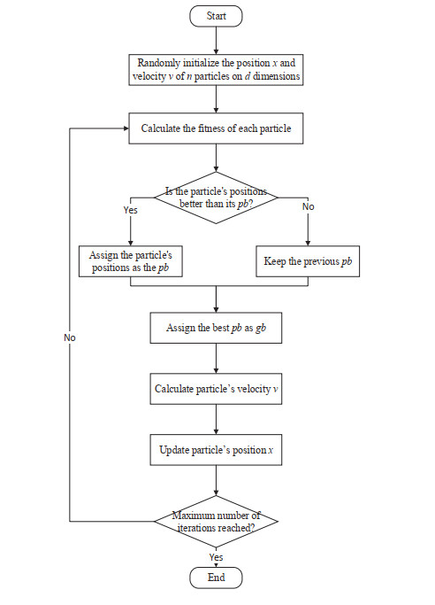
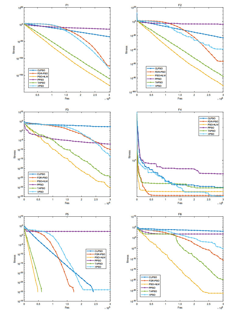
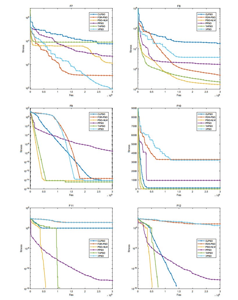
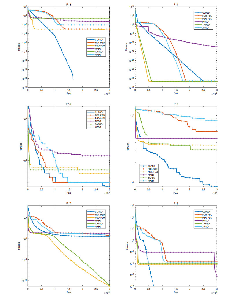
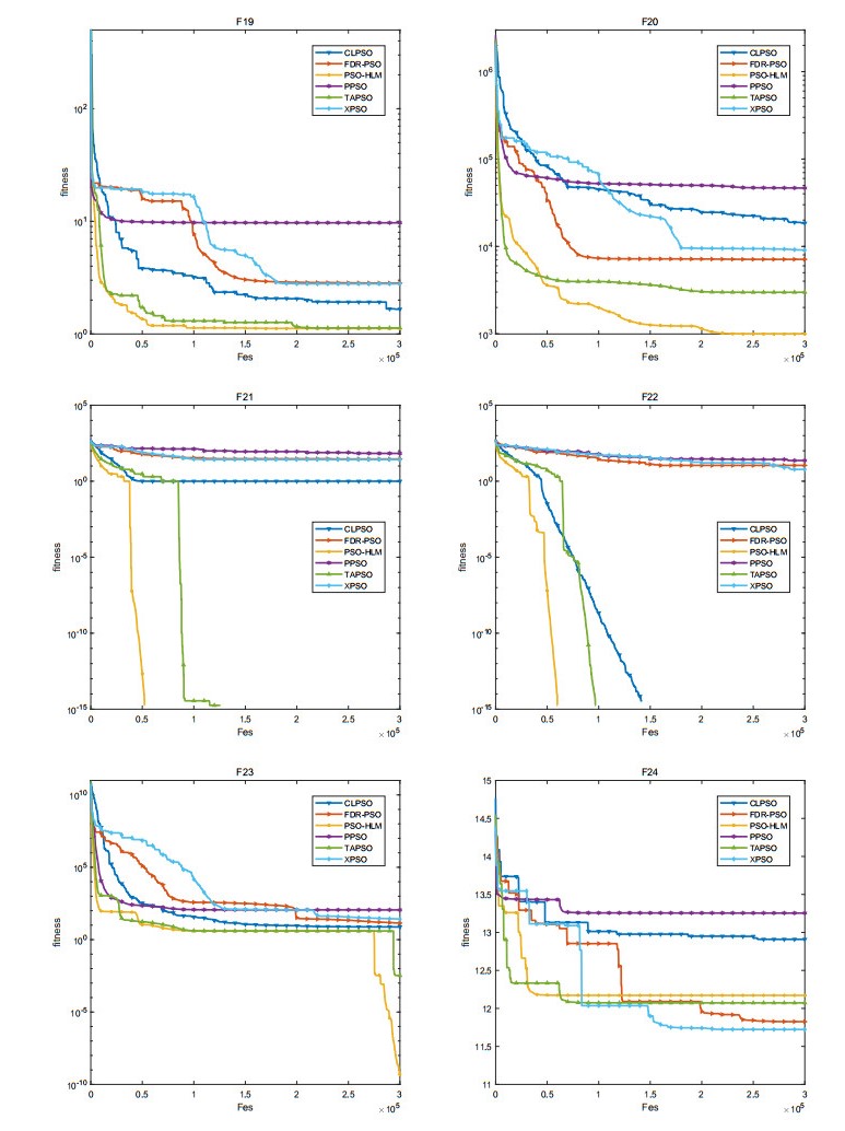
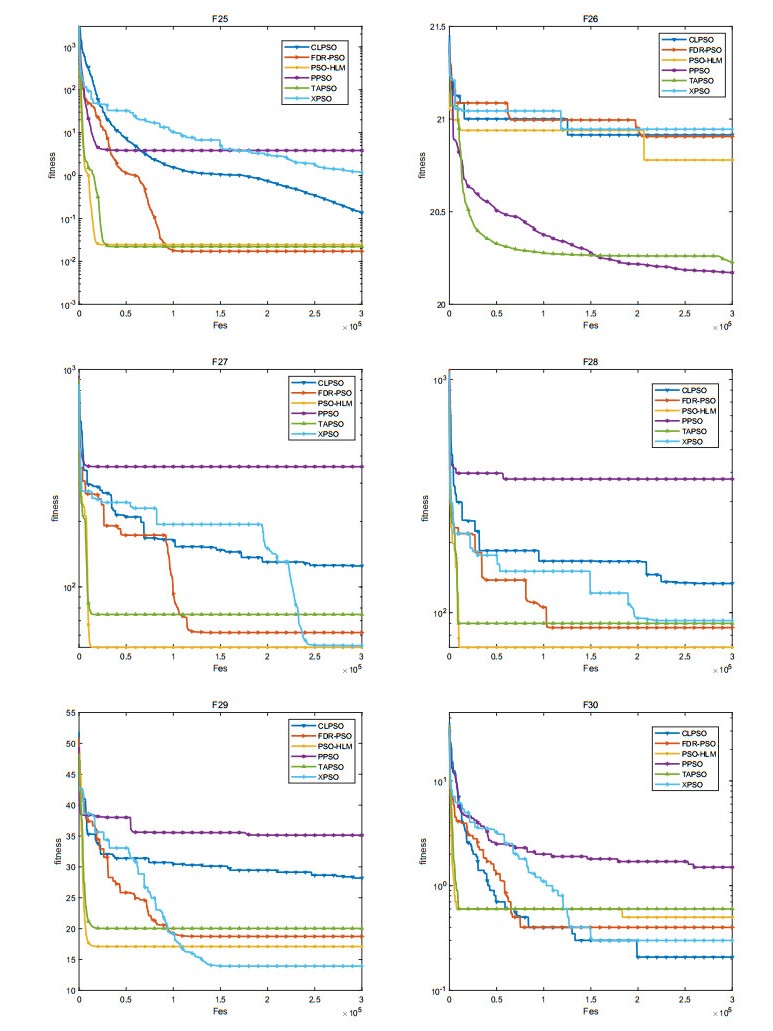
The convergence speed and the diversity of the population plays a critical role in the performance of particle swarm optimization (PSO). In order to balance the trade-off between exploration and exploitation, a novel particle swarm optimization based on the hybrid learning model (PSO-HLM) is proposed. In the early iteration stage, PSO-HLM updates the velocity of the particle based on the hybrid learning model, which can improve the convergence speed. At the end of the iteration, PSO-HLM employs a multi-pools fusion strategy to mutate the newly generated particles, which can expand the population diversity, thus avoid PSO-HLM falling into a local optima. In order to understand the strengths and weaknesses of PSO-HLM, several experiments are carried out on 30 benchmark functions. Experimental results show that the performance of PSO-HLM is better than other the-state-of-the-art algorithms.
Citation: Yufeng Wang, BoCheng Wang, Zhuang Li, Chunyu Xu. A novel particle swarm optimization based on hybrid-learning model[J]. Mathematical Biosciences and Engineering, 2023, 20(4): 7056-7087. doi: 10.3934/mbe.2023305
The convergence speed and the diversity of the population plays a critical role in the performance of particle swarm optimization (PSO). In order to balance the trade-off between exploration and exploitation, a novel particle swarm optimization based on the hybrid learning model (PSO-HLM) is proposed. In the early iteration stage, PSO-HLM updates the velocity of the particle based on the hybrid learning model, which can improve the convergence speed. At the end of the iteration, PSO-HLM employs a multi-pools fusion strategy to mutate the newly generated particles, which can expand the population diversity, thus avoid PSO-HLM falling into a local optima. In order to understand the strengths and weaknesses of PSO-HLM, several experiments are carried out on 30 benchmark functions. Experimental results show that the performance of PSO-HLM is better than other the-state-of-the-art algorithms.

| [1] |
G. G. Wang, S. Deb, Z. Cui, Monarch butterfly optimization, Neural Comput. Appl., 31 (2019), 1995–2014. https://doi.org/10.1007/s00521-015-1923-y doi: 10.1007/s00521-015-1923-y

|
| [2] |
S. Li, H. Chen, M. Wang, A. A. Heidari, S. Mirjalili, Slime mould algorithm: A new method for stochastic optimization, Future Gener. Comput. Syst., 111 (2020), 300–323. https://doi.org/10.1016/j.future.2020.03.055 doi: 10.1016/j.future.2020.03.055
|
| [3] |
C. G. Wang, Moth search algorithm: a bio-inspired metaheuristic algorithm for global optimization problems, Memetic Comput., 10 (2018), 151–164. https://doi.org/10.1007/s12293-016-0212-3 doi: 10.1007/s12293-016-0212-3
|
| [4] | Y. Yang, H. Chen, A. A. Heidari, A. Gandomi, Hunger games search: Visions, conception, implementation, deep analysis, perspectives, and towards performance shifts, Expert Syst. Appl., 177 (2021), 114864. |
| [5] |
J. C. Butcher, A history of Runge-Kutta methods, Appl. Numer. Math., 20 (1996), 247–260. https://doi.org/10.1016/0168-9274(95)00108-5 doi: 10.1016/0168-9274(95)00108-5
|
| [6] | J. Tu, H. Chen, M. Wang, A. H. Gandomi, The colony predation algorithm, J. Bionic Eng., 18 (2021), 674–710. |
| [7] |
I. Ahmadianfar, A. A. Heidari, S. Noshadian, H. Chen, A. H. Gandomi, INFO: An efficient optimization algorithm based on weighted mean of vectors, Expert Syst. Appl., 195 (2022), 116516. https://doi.org/10.1016/j.eswa.2022.116516 doi: 10.1016/j.eswa.2022.116516
|
| [8] |
A. A. Heidari, S. Mirjalili, H. Faris, I. Aljarah, M. Mafarja, H. Chen, Harris hawks optimization: Algorithm and applications, Future Gener. Comput. Syst., 97 (2019), 849–872. https://doi.org/10.1016/j.future.2019.02.028 doi: 10.1016/j.future.2019.02.028
|
| [9] | J. Kennedy, R. Eberhart, Particle swarm optimization, in Proceedings of ICNN'95-international conference on neural networks, (1995), 1942–1948. |
| [10] | X. J. Yang, Q. J. Jiao, X. Liu, Center particle swarm optimization algorithm, in 2019 IEEE 3rd Information Technology, Networking, Electronic and Automation Control Conference (ITNEC), (2019), 2084–2087. |
| [11] |
B. Wei, X. Xia, F. Yu, Y. Zhang, X. Xu, H. Wu, et al., Multiple adaptive strategies based particle swarm optimization algorithm, Swarm Evol. Comput., 57 (2020), 100731. https://doi.org/10.1016/j.swevo.2020.100731 doi: 10.1016/j.swevo.2020.100731
|
| [12] |
N. Lynn, P. N. Suganthan, Ensemble particle swarm optimizer, Appl. Soft Comput., 55 (2017), 533–548. https://doi.org/10.1016/j.asoc.2017.02.007 doi: 10.1016/j.asoc.2017.02.007
|
| [13] |
Cao H, Zheng H, Hu G. Generation of quasi-developable Q-Bezier strip via PSO-based shape parameters optimization, Math. Methods Appl. Sci., 45 (2022), 1118–1129. https://doi.org/10.1002/mma.7839 doi: 10.1002/mma.7839
|
| [14] | Q. Cui, C. Tang, G. Xu, C. Wu, X. Shi, Y. Liang, et al., Surprisingly popular algorithm-based comprehensive adaptive topology learning PSO, in 2019 IEEE Congress on Evolutionary Computation (CEC), (2019), 2603–2610. https://doi.org/10.1109/CEC.2019.8790002 |
| [15] | A. P. Engelbrecht, B. S. Masiye, G. Pampard, Niching ability of basic particle swarm optimization algorithms, in Proceedings 2005 IEEE Swarm Intelligence Symposium, (2005), 397–400. |
| [16] | Dong H, Zhang H, Han S, X. Li, X. Wang, Reverse-learning particle swarm optimization algorithm based on niching technology, in 2018 IEEE/ACIS 17th international conference on computer and information science (ICIS), (2018), 405–410. |
| [17] | Z. Du, S. Li, Y. Sun Y, N. Li, Adaptive particle swarm optimization algorithm based on levy flights mechanism, in 2017 Chinese Automation Congress (CAC), (2017), 479–484. |
| [18] |
X. Xia, L. Gui, F. Yu, H. Wu, B. Wei, Y. Zhang, et al., Triple archives particle swarm optimization, IEEE Trans. Cybern., 50 (2019), 4862–4875. https://doi.org/10.1109/TCYB.2019.2943928 doi: 10.1109/TCYB.2019.2943928
|
| [19] | D. K. Kole, A. Halder, An efficient dynamic image segmentation algorithm using a hybrid technique based on particle swarm optimization and genetic algorithm, in 2010 International Conference on Advances in Computer Engineering, (2010), 252–255. |
| [20] | A. Colorni, M. Dorigo, V. Maniezzo, Distributed optimization by ant colonies. Proceedings of the First European Conference on Artificial Life, (1998), 134–142. |
| [21] | R. C. Eberhart, J. Kennedy, A new optimiser using particle swarm theory, in Proceedings of the Sixth International Symposium on Micro Machine and Human Science, IEEE, (1995), 39–43. |
| [22] |
Liang J J, Qin A K, Suganthan P N, et al. Comprehensive learning particle swarm optimizer for global optimization of multimodal functions, IEEE Trans. Evol. Comput., 10 (2006), 281–295. https://doi.org/10.1109/TEVC.2005.857610 doi: 10.1109/TEVC.2005.857610
|
| [23] | O. M. Sedeh, B. Ostadi, F. Zagia, A novel hybrid GA-PSO optimization technique for multi-location facility maintenance scheduling problem, J. Build. Eng., 40 (2021), 102348. |
| [24] | M. Gao, Y. Zhu, J. Sun, The multi-objective cloud tasks scheduling based on hybrid particle swarm optimization, in 2020 Eighth International Conference on Advanced Cloud and Big Data (CBD), (2020). |
| [25] | X. Liu, H. Yi, Z. Ni, Application of ant colony optimization algorithm in process planning optimization, in 2012 Fifth International Conference on Intelligent Networks and Intelligent Systems, (2012), 61–64. https://doi.org/10.1111/j.1365-2559.2012.04359_7.x |
| [26] | S. Kefi, N. Rokbani, P. Kromer, A. M. Alimi, Ant supervised by PSO and 2-opt algorithm, AS-PSO-2Opt, applied to traveling salesman problem, in 2016 IEEE International Conference on Systems, Man, and Cybernetics (SMC), (2016), 4866–4871. https://doi.org/10.1109/SMC.2016.7844999 |
| [27] |
J. Lu, J. Zhang, J. Sheng, Enhanced multi-swarm cooperative particle swarm optimizer, Swarm Evol. Comput., 69 (2022), 100989. https://doi.org/10.1016/j.swevo.2021.100989 doi: 10.1016/j.swevo.2021.100989
|
| [28] | Y. Wang, W. Dong, X. Dong, Cooperative Coevolution with Correlation Learning Between Variables for Large Scale Overlapping Problem, Acta Electon. Sin., 48 (2018), 529. |
| [29] | Y. Gao, An improved hybrid group intelligent algorithm based on artificial bee colony and particle swarm optimization, in 2018 International Conference on Virtual Reality and Intelligent Systems (ICVRIS), (2018), 160–163. |
| [30] |
O. Ramos-Figueroa, M. Quiroz-Castellanos, E. Mezura-Montes, R. Kharel, Variation operators for grouping genetic algorithms: A review, Swarm Evol. Comput., 60 (2021), 100796. https://doi.org/10.1016/j.swevo.2020.100796 doi: 10.1016/j.swevo.2020.100796
|
| [31] |
A. Ratnaweera, S. K. Halgamuge, H. C. Watson, Self-organizing hierarchical particle swarm optimizer with time-varying acceleration coefficients, IEEE Trans. Evol. Comput., 8 (2004), 240–255. https://doi.org/10.1109/TEVC.2004.826071 doi: 10.1109/TEVC.2004.826071
|
| [32] | T. Peram, K. Veeramachaneni, C. K. Mohan, Fitness-distance-ratio based particle swarm optimization, in Proceedings of the 2003 IEEE Swarm Intelligence Symposium, (2003), 174–181. |
| [33] | J. Kennedy, R. Mendes, Population structure and particle swarm performance, in Proceedings of the 2002 Congress on Evolutionary Computation, (2002), 1671–1676. |
| [34] | T. Hayashida, I. Nishizaki, S. Sekizaki, Y. Takamori, Improvement of Particle Swarm Optimization Focusing on Diversity of the Particle Swarm, in 2020 IEEE International Conference on Systems, Man, and Cybernetics (SMC), (2020), 191–197. |
| [35] |
X. Xia, L. Gui, G. He, B. Wei, Y. Zhang, F. Yu, et al., An expanded particle swarm optimization based on multi-exemplar and forgetting ability, Inf. Sci., 508 (2020), 105–120. https://doi.org/10.1016/j.ins.2019.08.065 doi: 10.1016/j.ins.2019.08.065
|
| [36] |
X. Jin, Y. Liang, D. Tian, F. Zhuang, Particle swarm optimization using dimension selection methods, Appl. Math. Comput., 219 (2013), 5185–5197. https://doi.org/10.1016/j.amc.2012.11.020 doi: 10.1016/j.amc.2012.11.020
|
| [37] |
Y. Wang, W. Dong, X. Dong, A novel ITO Algorithm for influence maximization in the large-scale social networks, Future Gener. Comput. Syst., 88 (2018), 755–763. https://doi.org/10.1016/j.future.2018.04.026 doi: 10.1016/j.future.2018.04.026
|
| [38] | M. Ghasemi, E. Akbari, A. Rahimnejad, S. E. Razavi, S. Ghavidel, L. Li, Phasor particle swarm optimization: a simple and efficient variant of PSO, Soft Comput., 23 (2019), 9701–9718. |
Figures(6) / Tables(10)

Yufeng Wang, BoCheng Wang, Zhuang Li, Chunyu Xu. A novel particle swarm optimization based on hybrid-learning model[J]. Mathematical Biosciences and Engineering, 2023, 20(4): 7056-7087. doi: 10.3934/mbe.2023305


 DownLoad: