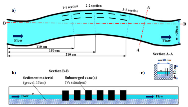
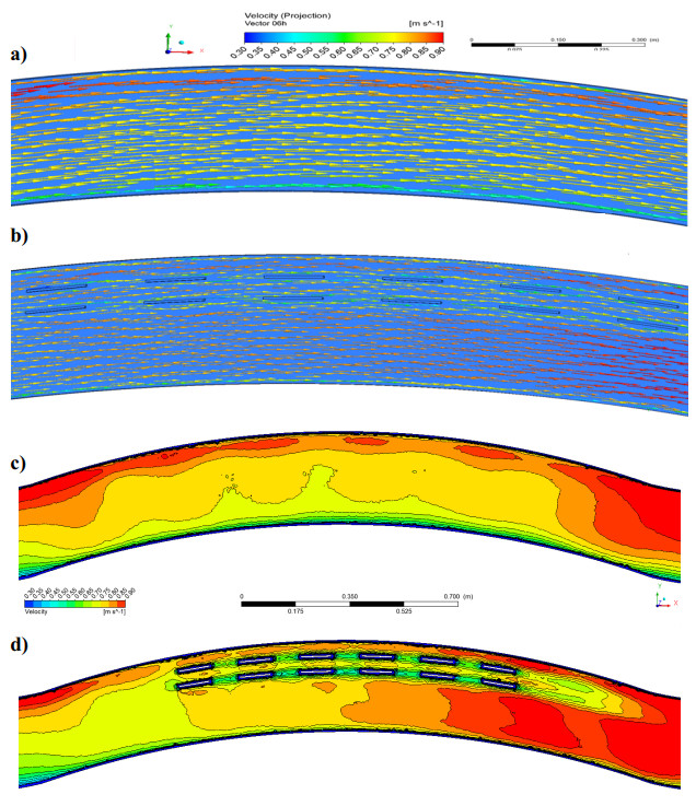
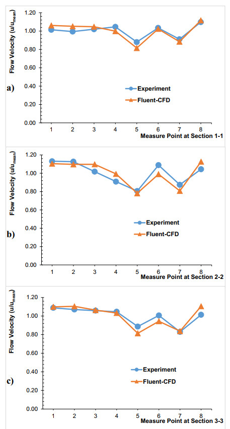
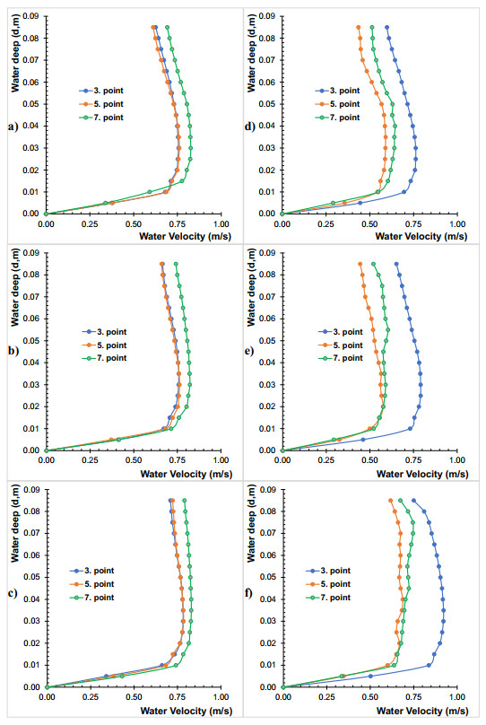
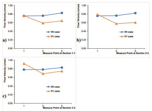
In the case of flooding in rivers, river regulation structures are important since scours occur on the outer meander due to high flow velocities. In this study, 2-array submerged vane structures were investigated which is a new method in the meandering part of open channels, both laboratory and numerically with an open channel flow discharge of 20 L/s. Open channel flow experiments were carried out by using a submerged vane and without a vane. The flow velocity results of the computational fluid dynamics (CFD) models were compared to the experimental results and the results were found compatible. The flow velocities were investigated along with depth using the CFD and found that the maximum velocity was reduced by 22–27% along the depth. In the outer meander, the 2-array submerged vane with a 6-vane structure was found to affect the flow velocity by 26–29% in the region behind the vane.
Citation: Bestami TAŞAR, Fatih ÜNEŞ, Ercan GEMİCİ. Laboratory and numerical investigation of the 2-array submerged vanes in meandering open channel[J]. Mathematical Biosciences and Engineering, 2023, 20(2): 3261-3281. doi: 10.3934/mbe.2023153
In the case of flooding in rivers, river regulation structures are important since scours occur on the outer meander due to high flow velocities. In this study, 2-array submerged vane structures were investigated which is a new method in the meandering part of open channels, both laboratory and numerically with an open channel flow discharge of 20 L/s. Open channel flow experiments were carried out by using a submerged vane and without a vane. The flow velocity results of the computational fluid dynamics (CFD) models were compared to the experimental results and the results were found compatible. The flow velocities were investigated along with depth using the CFD and found that the maximum velocity was reduced by 22–27% along the depth. In the outer meander, the 2-array submerged vane with a 6-vane structure was found to affect the flow velocity by 26–29% in the region behind the vane.

| [1] |
S. Chamran, G. A. Barani, M. S. Sardo, Experimental investigation of submerged vanes shape effect on river-bend stability, J. Hydraul. Struct., 1 (2013), 37–43. https://doi.org/10.22055/JHS.2013.10073 doi: 10.22055/JHS.2013.10073

|
| [2] |
A. Voisin, R. D. Townsend, Model testing of submerged vanes in strongly curved narrow channel bends, Can. J. Civil Eng., 29 (2002), 37–49. https://doi.org/10.1139/L01-078 doi: 10.1139/l01-078
|
| [3] |
K. Blanckaert, W. H. Graf, Momentum transport in sharp open-channel bends, J. Hydraul. Eng., 130 (2004), 186–198. https://doi.org/10.1061/(ASCE)0733-9429(2004)130:3(186) doi: 10.1061/(ASCE)0733-9429(2004)130:3(186)
|
| [4] |
A. J. Odgaard, J. F. Kennedy, River‐bend bank protection by submerged vanes, J. Hydraul. Eng., 109 (1983), 1161–1173. https://doi.org/10.1061/(ASCE)0733-9429(1983)109:8(1161) doi: 10.1061/(ASCE)0733-9429(1983)109:8(1161)
|
| [5] | A. J. Odgaard, J. F. Kennedy, Analysis of Sacramento River Bend Flows, and Development of a New Method for Bank Protection, Iowa, 1982. |
| [6] |
B. Ghorbani, J. A. Kells, Effect of submerged vanes on the scour occurring at a cylindrical pier, J. Hydraul. Res., 46 (2010), 610–619. https://doi.org/10.3826/JHR.2008.3003 doi: 10.3826/JHR.2008.3003
|
| [7] | L. Davoodi, M. S. Bejestan, International control of sediment entry to intake on a trapezoidal channel by submerged vane, Ecol. Environ. Conserv., 18 (2012), 165–169. |
| [8] | E. Gemici, Flow management with submerged vanes in open channels, Erciyes University, Graduate School of Natural and Applied Sciences, Ph.D. Thesis, 2015. |
| [9] |
S. Mohammadiun, S. A. A. Salehi Neyshabouri, G. Naser, H. Vahabi, Numerical investigation of submerged vane effects on flow pattern in a 90° junction of straight and bend open channels, Iran. J. Sci. Technol., Trans. Civil Eng., 40 (2016), 349–365. https://doi.org/10.1007/s40996-016-0039-7 doi: 10.1007/s40996-016-0039-7
|
| [10] |
A. Fathi, S. M. A. Zomorodian, Effect of submerged vanes on scour around a bridge abutment, KSCE J. Civil Eng., 22 (2018), 2281–2289. https://doi.org/10.1007/s12205-017-1453-5 doi: 10.1007/s12205-017-1453-5
|
| [11] |
S. T. Kalathil, A. Wuppukondur, R. K. Balakrishnan, V. Chandra, Control of sediment inflow into a trapezoidal intake canal using submerged vanes, J. Waterw. Port Coastal Ocean Eng., 144 (2018), 04018020. https://doi.org/10.1061/(ASCE)WW.1943-5460.0000474 doi: 10.1061/(ASCE)WW.1943-5460.0000474
|
| [12] |
E. Zarei, M. Vaghefi, S. S. Hashemi, Bed topography variations in bend by simultaneous installation of submerged vanes and single bridge pier, Arabian J. Geosci., 12 (2019), 1–10. https://doi.org/10.1007/S12517-019-4342-Z/TABLES/2 doi: 10.1007/s12517-018-4128-8
|
| [13] |
M. Karami Moghadam, A. Amini, A. Keshavarzi, Intake design attributes and submerged vanes effects on sedimentation and shear stress, Water Environ. J., 34 (2020), 374–380. https://doi.org/10.1111/WEJ.12471 doi: 10.1111/wej.12471
|
| [14] |
R. Azizi, S. Bajestan, Iranian hydraulic association journal of hydraulics performance evaluation of submerged vanes by flow-3D numerical model, J. Hydraul., 15 (2020), 1–11. https://doi.org/10.30482/JHYD.2020.105497 doi: 10.30482/JHYD.2020.105497
|
| [15] |
J. Baltazar, E. Alves, G. Bombar, A. H. Cardoso, Effect of a submerged vane-field on the flow pattern of a movable bed channel with a 90 lateral diversion, Water, 13 (2021), 828. https://doi.org/10.3390/w13060828 doi: 10.3390/w13060828
|
| [16] |
R. W. Lake, S. Shaeri, S. T. M. L. D. Senevirathna, Design of submerged vane matrices to accompany a river intake in Australia, J. Environ. Eng. Sci., 16 (2021), 58–65. https://doi.org/10.1680/jenes.19.00037 doi: 10.1680/jenes.19.00037
|
| [17] |
R. R. W. Affonso, R. S. F. Dam, W. L. Salgado, A. X. da Silva, C. M. Salgado, Flow regime and volume fraction identification using nuclear techniques, artificial neural networks and computational fluid dynamics, Appl. Radiat. Isot., 159 (2020), 109103. https://doi.org/10.1016/J.APRADISO.2020.109103 doi: 10.1016/j.apradiso.2020.109103
|
| [18] |
P. P. Gadge, V. Jothiprakash, V. V. Bhosekar, Hydraulic investigation and design of roof profile of an orifice spillway using experimental and numerical models, J. Appl. Water Eng. Res., 6 (2016), 85–94. https://doi.org/10.1080/23249676.2016.1214627 doi: 10.1080/23249676.2016.1214627
|
| [19] |
F. Unes, H. Varcin, 3-D real dam reservoir model for seasonal thermal density flow, Environ. Eng. Manage. J., 16 (2017), 2009–2024. https://doi.org/10.30638/eemj.2017.209 doi: 10.30638/eemj.2017.209
|
| [20] | F. Üneş, M. Demirci, H. Varçin, 3-D numerical simulation of a real dam reservoir: Thermal stratified flow, in Advances in Hydroinformatics, Springer, Singapore, (2016), 377–394. https://doi.org/10.1007/978-981-287-615-7_26 |
| [21] |
N. Penna, M. de Marchis, O. B. Canelas, E. Napoli, A. H. Cardoso, R. Gaudio, Effect of the junction angle on turbulent flow at a hydraulic confluence, Water, 10 (2018), 469. https://doi.org/10.3390/W10040469 doi: 10.3390/w10040469
|
| [22] |
F. Salmasi, A. Samadi, Experimental and numerical simulation of flow over stepped spillways, Appl. Water Sci., 8 (2018), 1–11. https://doi.org/10.1007/S13201-018-0877-5/TABLES/3 doi: 10.1007/s13201-017-0639-9
|
| [23] |
E. Gabreil, S. J. Tait, S. Shao, A. Nichols, SPHysics simulation of laboratory shallow free surface turbulent flows over a rough bed, J. Hydraul. Res., 56 (2018), 727–747. https://doi.org/10.1080/00221686.2017.1410732 doi: 10.1080/00221686.2017.1410732
|
| [24] |
E. Gabreil, H. Wu, C. Chen, J. Li, M. Rubinato, X. Zheng, et al., Three-dimensional smoothed particle hydrodynamics modeling of near-shore current flows over rough topographic surface, Front. Mar. Sci., 9 (2022), 935098. https://doi.org/10.3389/fmars.2022.935098 doi: 10.3389/fmars.2022.935098
|
| [25] | A. J. Odgaard, River channel stabilization with submerged vanes, in Advances in Water Resources Engineering, Springer International Publishing, Cham, (2015), 107–136. https://doi.org/10.1007/978-3-319-11023-3_3 |
| [26] |
E. Turhan, H. Ozmen-Cagatay, S. Kocaman, Experimental and numerical investigation of shock wave propagation due to dam-break over a wet channel, Pol. J. Environ. Stud., 28 (2019), 2877–2898. https://doi.org/10.15244/pjoes/92824 doi: 10.15244/pjoes/92824
|
| [27] |
H. Ozmen-Cagatay, E. Turhan, S. Kocaman, An experimental investigation of dam-break induced flood waves for different density fluids, Ocean Eng., 243 (2022), 110227. https://doi.org/10.1016/J.OCEANENG.2021.110227 doi: 10.1016/j.oceaneng.2021.110227
|
| [28] | B. E. Launder, D. B. Spalding, Mathematical Models of Turbulence, Academic Press, New York, 1972. |
| [29] |
H. Kim, P. Nanjundan, Y. W. Lee, Numerical study on the sloshing flows in a prismatic tank using natural frequency of the prismatic shapes, Prog. Comput. Fluid Dyn., 21 (2021), 152–160. https://doi.org/10.1504/PCFD.2021.115129 doi: 10.1504/PCFD.2021.115129
|
| [30] |
O. Simsek, M. S. Akoz, N. G. Soydan, Numerical validation of open channel flow over a curvilinear broad-crested weir, Prog. Comput. Fluid Dyn., 16 (2016), 364–378. https://doi.org/10.1504/PCFD.2016.080055 doi: 10.1504/PCFD.2016.080055
|
| [31] |
C. W. Hirt, B. D. Nichols, Volume of fluid (VOF) method for the dynamics of free boundaries, J. Comput. Phys., 39 (1981), 201–225. https://doi.org/10.1016/0021-9991(81)90145-5 doi: 10.1016/0021-9991(81)90145-5
|
| [32] |
S. M. Salim, M. Ariff, S. C. Cheah, Wall y+ approach for dealing with turbulent flows over a wall mounted cube, Prog. Comput. Fluid Dyn., 10 (2010), 341–351. https://doi.org/10.1504/PCFD.2010.035368 doi: 10.1504/PCFD.2010.035368
|
| [33] | A. Gerasimov, Modeling Turbulent Flows with Fluent, presentation, Seminar on Turbulence Modelling for FLUENT users, 2006. Avalible from: http://www.ae.metu.edu.tr/seminar/Turbulence_Seminar/Modelling_turbulent_flows_with_FLUENT.pdf. |
| [34] |
A. J. Odgaard, River training and sediment management with submerged vanes, Am. Soc. Civil Eng., 2009 (2009). https://doi.org/10.1061/9780784409817 doi: 10.1061/9780784409817
|
| [35] |
P. Biswas, A. K. Barbhuiya, Effect of submerged vane on three dimensional flow dynamics and bed morphology in river bend, River Res. Appl., 35 (2019), 301–312. https://doi.org/10.1002/rra.3402 doi: 10.1002/rra.3402
|
Figures(12) / Tables(4)

Bestami TAŞAR, Fatih ÜNEŞ, Ercan GEMİCİ. Laboratory and numerical investigation of the 2-array submerged vanes in meandering open channel[J]. Mathematical Biosciences and Engineering, 2023, 20(2): 3261-3281. doi: 10.3934/mbe.2023153


 DownLoad: