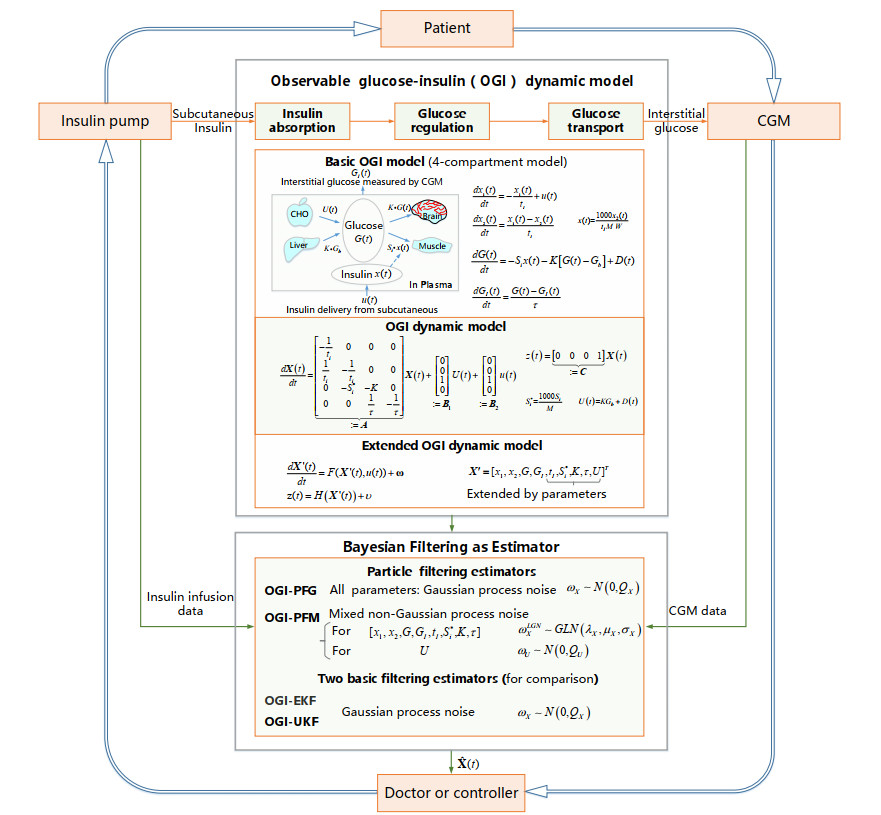
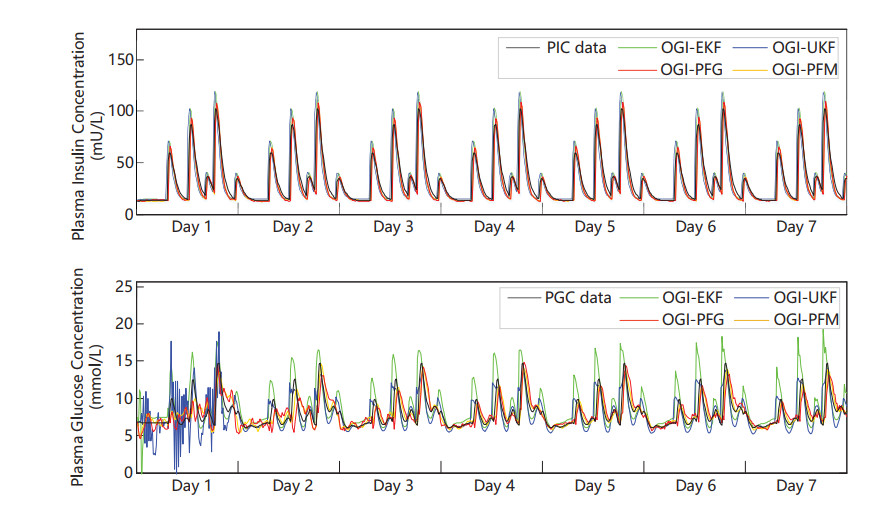
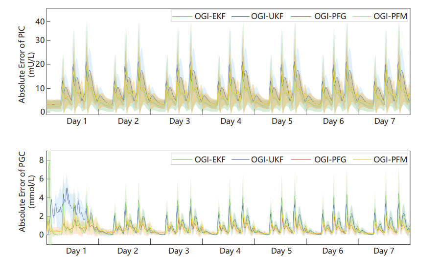
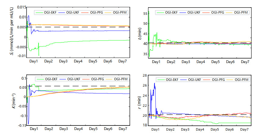
Plasma glucose concentration (PGC) and plasma insulin concentration (PIC) are two essential metrics for diabetic regulation, but difficult to be measured directly. Often, PGC and PIC are estimated from continuous glucose monitoring and insulin delivery data. Nevertheless, the inter-individual variability and external disturbance (e.g. carbohydrate intake) bring challenges for accurate estimations. This study is to estimate PGC and PIC adaptively by identifying personalized parameters and external disturbances. An observable glucose-insulin (OGI) dynamic model is established to describe insulin absorption, glucose regulation, and glucose transport. The model parameters and disturbances can be extended to observable state variables and be identified dynamically by Bayesian filtering estimators. Two basic Gaussian noise based Bayesian filtering estimators, extended Kalman filtering (EKF) and unscented Kalman filtering (UKF), are implemented. Recognizing the prevalence of non-Gaussian noise, in this study, two new filtering estimators: particle filtering with Gaussian noise (PFG), and particle filtering with mixed non-Gaussian noise (PFM) are designed and implemented. The proposed OGI model in conjunction with the estimators is evaluated using the data from 30 in-silico subjects and 10 human participants. For in-silico subjects, the OGI with PFM estimator has the ability to estimate PIC and PGC adaptively, achieving RMSE of PIC $ 9.49\pm3.81 $ mU/L, and PGC $ 0.89\pm0.19 $ mmol/L. For human, the OGI with PFM has the promise to identify disturbances ($ 95.46\%\pm0.65\% $ accurate rate of meal identification). OGI model provides a way to fully personalize the parameters and external disturbances in real time, and has potential clinical utility for artificial pancreas.
Citation: Weijie Wang, Shaoping Wang, Yixuan Geng, Yajing Qiao, Teresa Wu. An OGI model for personalized estimation of glucose and insulin concentration in plasma[J]. Mathematical Biosciences and Engineering, 2021, 18(6): 8499-8523. doi: 10.3934/mbe.2021420
Plasma glucose concentration (PGC) and plasma insulin concentration (PIC) are two essential metrics for diabetic regulation, but difficult to be measured directly. Often, PGC and PIC are estimated from continuous glucose monitoring and insulin delivery data. Nevertheless, the inter-individual variability and external disturbance (e.g. carbohydrate intake) bring challenges for accurate estimations. This study is to estimate PGC and PIC adaptively by identifying personalized parameters and external disturbances. An observable glucose-insulin (OGI) dynamic model is established to describe insulin absorption, glucose regulation, and glucose transport. The model parameters and disturbances can be extended to observable state variables and be identified dynamically by Bayesian filtering estimators. Two basic Gaussian noise based Bayesian filtering estimators, extended Kalman filtering (EKF) and unscented Kalman filtering (UKF), are implemented. Recognizing the prevalence of non-Gaussian noise, in this study, two new filtering estimators: particle filtering with Gaussian noise (PFG), and particle filtering with mixed non-Gaussian noise (PFM) are designed and implemented. The proposed OGI model in conjunction with the estimators is evaluated using the data from 30 in-silico subjects and 10 human participants. For in-silico subjects, the OGI with PFM estimator has the ability to estimate PIC and PGC adaptively, achieving RMSE of PIC $ 9.49\pm3.81 $ mU/L, and PGC $ 0.89\pm0.19 $ mmol/L. For human, the OGI with PFM has the promise to identify disturbances ($ 95.46\%\pm0.65\% $ accurate rate of meal identification). OGI model provides a way to fully personalize the parameters and external disturbances in real time, and has potential clinical utility for artificial pancreas.

| [1] | M. A. Atkinson, G. S. Eisenbarth, A. W. Michels, Type 1 diabetes, The Lancet, 383 (2014), 69–82. |
| [2] |
A. D. Association, Diagnosis and classification of diabetes mellitus, Diabetes Care, 33 (2010), S62–S69. doi: 10.2337/dc10-S062

|
| [3] | C. Cobelli, C. Dalla Man, G. Sparacino, L. Magni, G. De Nicolao, B. P. Kovatchev, Diabetes: Models, signals, and control, IEEE Rev. Biomed. Eng., 2 (2009), 54–96. |
| [4] |
T. Danne, R. Nimri, T. Battelino, R. M. Bergenstal, K. L. Close, et al., International consensus on use of continuous glucose monitoring, Diabetes Care, 40 (2017), 1631–1640. doi: 10.2337/dc17-1600
|
| [5] |
S. V. Edelman, N. B. Argento, J. Pettus, I. B. Hirsch, Clinical implications of real-time and intermittently scanned continuous glucose monitoring, Diabetes Care, 41 (2018), 2265–2274. doi: 10.2337/dc18-1150
|
| [6] | L. Heinemann, G. A. Fleming, J. R. Petrie, R. W. Holl, R. M. Bergenstal, A. L. Peters, Insulin pump risks and benefits: a clinical appraisal of pump safety standards, adverse event reporting, and research needs, Diabetes Care, 38 (2015), 716–722. |
| [7] |
S. Brown, D. Raghinaru, E. Emory, B. Kovatchev, First look at Control-IQ: a new-generation automated insulin delivery system, Diabetes Care, 41 (2018), 2634–2636. doi: 10.2337/dc18-1249
|
| [8] |
E. Atlas, R. Nimri, S. Miller, E. A. Grunberg, M. Phillip, MD-logic artificial pancreas system: a pilot study in adults with type 1 diabetes, Diabetes Care, 33 (2010), 1072–1076. doi: 10.2337/dc09-1830
|
| [9] |
K. Turksoy, E. Littlejohn, A. Cinar, Multimodule, multivariable artificial pancreas for patients with type 1 diabetes: Regulating glucose concentration under challenging conditions, IEEE Control Syst. Mag., 38 (2018), 105–124. doi: 10.1109/MCS.2017.2766326
|
| [10] |
S. O'Neill, Update on technologies, medicines and treatments, Diabet. Med. J. British Diabetes Assoc., 37 (2020), 709–711. doi: 10.1111/dme.14229
|
| [11] |
G. E. Umpierrez, D. C. Klonoff, Diabetes technology update: Use of insulin pumps and continuous glucose monitoring in the hospital, Diabetes Care, 41 (2018), 1579–1589. doi: 10.2337/dci18-0002
|
| [12] |
J. Bondia, S. Romero-Vivo, B. Ricarte, J. L. Diez, Insulin estimation and prediction: A review of the estimation and prediction of subcutaneous insulin pharmacokinetics in closed-loop glucose control, IEEE Control Syst. Mag., 38 (2018), 47–66. doi: 10.1109/MCS.2017.2766312
|
| [13] |
J. Pickup, H. Keen, Continuous subcutaneous insulin infusion at 25 years: evidence base for the expanding use of insulin pump therapy in type 1 diabetes, Diabetes Care, 25 (2002), 593–598. doi: 10.2337/diacare.25.3.593
|
| [14] |
I. Hajizadeh, M. Rashid, S. Samadi, M. Sevil, A. Cinar, Adaptive personalized multivariable artificial pancreas using plasma insulin estimates, J. Process Control, 80 (2019), 26–40. doi: 10.1016/j.jprocont.2019.05.003
|
| [15] |
C. Neatpisarnvanit, J. R. Boston, Estimation of plasma insulin from plasma glucose, IEEE Transact. Biomed. Eng., 49 (2002), 1253–1259. doi: 10.1109/TBME.2002.804599
|
| [16] |
C. M. Ramkissoon, P. Herrero, J. Bondia, J. Vehi, Unannounced meals in the artificial pancreas: Detection using continuous glucose monitoring, Sensors, 18 (2018), 884–901. doi: 10.3390/s18030884
|
| [17] | L. O. Avila, M. De Paula, C. R. Sanchez-Reinoso, Estimation of plasma insulin concentration under glycemic variability using nonlinear filtering techniques, Biosystems, 171 (2018), 1–9. |
| [18] |
D. de Pereda, S. Romero-Vivo, B. Ricarte, P. Rossetti, F. J. Ampudia-Blasco, J. Bondia, Real-time estimation of plasma insulin concentration from continuous glucose monitor measurements, Computer Methods Biomech. Biomed. Eng., 19 (2016), 934–942. doi: 10.1080/10255842.2015.1077234
|
| [19] |
K. Turksoy, I. Hajizadeh, S. Samadi, J. Feng, M. Sevil, et al., Real-time insulin bolusing for unannounced meals with artificial pancreas, Control Eng. Pract., 59 (2017), 159–164. doi: 10.1016/j.conengprac.2016.08.001
|
| [20] |
A. C. Charalampidis, K. Pontikis, G. D. Mitsis, G. Dimitriadis, V. Lampadiari, et al., Calibration of a microdialysis sensor and recursive glucose level estimation in ICU patients using Kalman and particle filtering, Biomed. Signal Process. Control, 27 (2016), 155–163. doi: 10.1016/j.bspc.2015.11.003
|
| [21] |
I. Hajizadeh, M. Rashid, K. Turksoy, S. Samadi, J. Feng, et al., Plasma insulin estimation in people with type 1 diabetes mellitus, Indust. Eng. Chem. Res., 56 (2017), 9846–9857. doi: 10.1021/acs.iecr.7b01618
|
| [22] |
J. Ko, D. Fox, GP-BayesFilters: Bayesian filtering using Gaussian process prediction and observation models, Auton. Robot., 27 (2009), 75–90. doi: 10.1007/s10514-009-9119-x
|
| [23] | Y. Ruan, M. E. Wilinska, H. Thabit, R. Hovorka, Modeling day-to-day variability of glucose–insulin regulation over 12-week home use of closed-loop insulin delivery, IEEE Transact. Biomed. Eng., 64 (2016), 1412–1419. |
| [24] |
W. Wang, S. Wang, X. Wang, D. Liu, Y. Geng, T. Wu, A glucose-insulin mixture model and application to short-term hypoglycemia prediction in the night time, IEEE Transact. Biomed. Eng., 68 (2021), 834–845. doi: 10.1109/TBME.2020.3015199
|
| [25] |
W. Liu, A mathematical model for the robust blood glucose tracking, Math. Biosci. Eng., 16 (2019), 759–781. doi: 10.3934/mbe.2019036
|
| [26] |
K. Fessel, J. B. Gaither, J. K. Bower, T. Gaillard, K. Osei, G. A. Rempała, Mathematical analysis of a model for glucose regulation, Math. Biosci. Eng., 13 (2016), 83–99. doi: 10.3934/mbe.2016.13.83
|
| [27] |
H. F. Arguedas, M. A. Capistran, Bayesian analysis of glucose dynamics during the oral glucose tolerance test, Math. Biosci. Eng., 18 (2021), 4628-4647. doi: 10.3934/mbe.2021235
|
| [28] |
X. Shi, Q. Zheng, J. Yao, J. Li, X. Zhou, Analysis of a stochastic IVGTT glucose-insulin model with time delay, Math. Biosci. Eng., 17 (2020), 2310–2329. doi: 10.3934/mbe.2020123
|
| [29] |
N. Chopin, A sequential particle filter method for static models, Biometrika, 89 (2002), 539–552. doi: 10.1093/biomet/89.3.539
|
| [30] | J. Wei, G. Dong, Z. Chen, Remaining useful life prediction and state of health diagnosis for lithium-ion batteries using particle filter and support vector regression, IEEE Transact. Indust. Elect., 65 (2017), 5634–5643. |
| [31] |
M. S. Arulampalam, S. Maskell, N. Gordon, T. Clapp, A tutorial on particle filters for online nonlinear/non-Gaussian Bayesian tracking, IEEE Transact. Signal Process., 50 (2002), 174–188. doi: 10.1109/78.978374
|
| [32] |
R. N. Bergman, L. S. Phillips, C. Cobelli, Physiologic evaluation of factors controlling glucose tolerance in man: measurement of insulin sensitivity and beta-cell glucose sensitivity from the response to intravenous glucose, J. Clin. Invest., 68 (1981), 1456–1467. doi: 10.1172/JCI110398
|
| [33] |
A. De Gaetano, O. Arino, Mathematical modelling of the intravenous glucose tolerance test, J. Math. Biol., 40 (2000), 136–168. doi: 10.1007/s002850050007
|
| [34] | E. Horová, J. Mazoch, J. HiIgertová, J. Kvasnička, J. Škrha, et al., Acute hyperglycemia does not impair microvascular reactivity and endothelial function during hyperinsulinemic isoglycemic and hyperglycemic clamp in type 1 diabetic patients, Exper. Diabetes Res., 2012, 59–66. |
| [35] |
N. Magdelaine, L. Chaillous, I. Guilhem, J.-Y. Poirier, M. Krempf, et al., A long-term model of the glucose–insulin dynamics of type 1 diabetes, IEEE Transact. Biomed. Eng., 62 (2015), 1546–1552. doi: 10.1109/TBME.2015.2394239
|
| [36] |
R. Hermann, A. Krener, Nonlinear controllability and observability, IEEE Transact. Autom. Control, 22 (1977), 728–740. doi: 10.1109/TAC.1977.1101601
|
| [37] | Q. Ma, Structural conditions on observability of nonlinear systems, Int. J. Inform. Technol. Computer Sci., 3 (2011), 16–22. |
| [38] |
C. Yardim, Z. H. Michalopoulou, P. Gerstoft, An overview of sequential Bayesian filtering in ocean acoustics, IEEE J. Ocean. Eng., 36 (2011), 71–89. doi: 10.1109/JOE.2010.2098810
|
| [39] |
C. Eberle, C. Ament, The Unscented Kalman Filter estimates the plasma insulin from glucose measurement, Biosystems, 103 (2011), 67–72. doi: 10.1016/j.biosystems.2010.09.012
|
| [40] | T. Li, M. Bolic, P. M. Djuric, Resampling methods for particle filtering: classification, implementation, and strategies, IEEE Signal Proc. Mag., 32 (2015), 70–86. |
| [41] |
B. M. Hill, The three-parameter lognormal distribution and Bayesian analysis of a point-source epidemic, J. Am. Stat. Assoc., 58 (1963), 72–84. doi: 10.1080/01621459.1963.10500833
|
| [42] |
C. D. Man, F. Micheletto, D. Lv, M. Breton, B. Kovatchev, C. Cobelli, The UVA/PADOVA type 1 diabetes simulator: New features, J. Diabetes Sci. Technol., 8 (2014), 26–34. doi: 10.1177/1932296813514502
|
| [43] |
R. Visentin, C. Dalla Man, C. Cobelli, One-day Bayesian cloning of type 1 diabetes subjects: toward a single-day UVA/Padova type 1 diabetes simulator, IEEE Transact. Biomed. Eng., 63 (2016), 2416–2424. doi: 10.1109/TBME.2016.2535241
|
| [44] |
B. P. Kovatchev, M. Breton, C. D. Man, C. Cobelli, In silico preclinical trials: a proof of concept in closed-loop control of type 1 diabetes, J. Diabetes Sci. Technol., 3 (2009), 44–55. doi: 10.1177/193229680900300106
|
| [45] |
C. Cobelli, C. D. Man, M. G. Pedersen, A. Bertoldo, Advancing our understanding of the glucose system via modeling: A perspective, IEEE Transact. Biomed. Eng., 61 (2014), 1577–1592. doi: 10.1109/TBME.2014.2310514
|
| [46] |
S. Samadi, K. Turksoy, I. Hajizadeh, J. Feng, M. Sevil, A. Cinar, Meal detection and carbohydrate estimation using continuous glucose sensor data, IEEE J. Biomed. Health Inform., 21 (2017), 619–627. doi: 10.1109/JBHI.2017.2677953
|
| [47] | K. Turksoy, S. Samadi, J. Feng, E. Littlejohn, L. Quinn, A. Cinar, Meal detection in patients with type 1 diabetes: a new module for the multivariable adaptive artificial pancreas control system, IEEE J. Biomed. Health Inform., 20 (2015), 47–54. |
| [48] | M. Vettoretti, A. Facchinetti, G. Sparacino, C. Cobelli, Type-1 diabetes patient decision simulator for in silico testing safety and effectiveness of insulin treatments, IEEE Transact. Biomed. Eng., 65 (2017), 1281–1290. |
| [49] |
M. Breton, B. Kovatchev, Analysis, modeling, and simulation of the accuracy of continuous glucose sensors, J. Diabetes Sci. Technol., 2 (2008), 853–862. doi: 10.1177/193229680800200517
|
| [50] | D. J. Albers, M. Levine, B. Gluckman, H. Ginsberg, G. Hripcsak, L. Mamykina, Personalized glucose forecasting for type 2 diabetes using data assimilation, PLoS Comput. Biol., 13 (2017), 1–38. |
| [51] | F. Rahmanian, M. Dehghani, P. Karimaghaee, M. Mohammadi, R. Abolpour, Hardware-in-the-loop control of glucose in diabetic patients based on nonlinear time-varying blood glucose model, Biomed. Signal Process. Control, 66 (2021), 1–12. |
Figures(5) / Tables(8)

Weijie Wang, Shaoping Wang, Yixuan Geng, Yajing Qiao, Teresa Wu. An OGI model for personalized estimation of glucose and insulin concentration in plasma[J]. Mathematical Biosciences and Engineering, 2021, 18(6): 8499-8523. doi: 10.3934/mbe.2021420


 DownLoad: