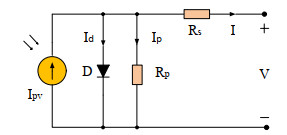
Photovoltaic (PV) parameter extraction plays a key role in establishing accurate and reliable PV models based on the manufacturer's current-voltage data. Owning to the characteristics such as implicit and nonlinear of the PV model, it remains a challenging and research-meaningful task in PV system optimization. Despite there are many methods that have been developed to solve this problem, they are often consuming a great deal of computing resources for more satisfactory results. To reduce computing resources, in this paper, an advanced differential evolution with search space decomposition is developed to effectively extract the unknown parameters of PV models. In proposed approach, a recently proposed advanced differential evolution algorithm is used as a solver. In addition, a search space decomposition technique is introduced to reduce the dimension of the problem, thereby reducing the complexity of the problem. Three different PV cell models are selected for verifying the performance of proposed approach. The experimental result is firstly compared with some representative differential evolution algorithms that do not use search space decomposition technique, which demonstrates the effectiveness of the search space decomposition. Moreover, the comparison results with some reported well-established parameter extraction methods suggest that the proposed approach not only obtains accurate and reliable parameters, but also uses the least computational resources.
Citation: Zhen Yan, Shuijia Li, Wenyin Gong. An adaptive differential evolution with decomposition for photovoltaic parameter extraction[J]. Mathematical Biosciences and Engineering, 2021, 18(6): 7363-7388. doi: 10.3934/mbe.2021364
Photovoltaic (PV) parameter extraction plays a key role in establishing accurate and reliable PV models based on the manufacturer's current-voltage data. Owning to the characteristics such as implicit and nonlinear of the PV model, it remains a challenging and research-meaningful task in PV system optimization. Despite there are many methods that have been developed to solve this problem, they are often consuming a great deal of computing resources for more satisfactory results. To reduce computing resources, in this paper, an advanced differential evolution with search space decomposition is developed to effectively extract the unknown parameters of PV models. In proposed approach, a recently proposed advanced differential evolution algorithm is used as a solver. In addition, a search space decomposition technique is introduced to reduce the dimension of the problem, thereby reducing the complexity of the problem. Three different PV cell models are selected for verifying the performance of proposed approach. The experimental result is firstly compared with some representative differential evolution algorithms that do not use search space decomposition technique, which demonstrates the effectiveness of the search space decomposition. Moreover, the comparison results with some reported well-established parameter extraction methods suggest that the proposed approach not only obtains accurate and reliable parameters, but also uses the least computational resources.

| [1] | T. Teo, T. Logenthiran, W. Woo, Forecasting of photovoltaic power using extreme learning machine, in 2015 IEEE Innovative Smart Grid Technologies - Asia (ISGT ASIA), (2015), 1–6. |
| [2] | V. De, T. Teo, W. Woo, T. Logenthiran, Photovoltaic power forecasting using lstm on limited dataset, in 2018 IEEE Innovative Smart Grid Technologies - Asia (ISGT Asia), (2018), 710–715. |
| [3] |
I. Ibrahim, M. Hossain, B. Duck, M. Nadarajah, An improved wind driven optimization algorithm for parameters identification of a triple-diode photovoltaic cell model, Energy Convers. Manage., 213 (2020), 112872. doi: 10.1016/j.enconman.2020.112872

|
| [4] |
Y. Zhang, M. Ma, Z. Jin, Comprehensive learning jaya algorithm for parameter extraction of photovoltaic models, Energy, 211 (2020), 118644. doi: 10.1016/j.energy.2020.118644
|
| [5] |
B. Dong, A. Luzin, D. Gura, The hybrid method based on ant colony optimization algorithm in multiple factor analysis of the environmental impact of solar cell technologies, Math. Biosci. Eng., 17 (2020), 6342–6354. doi: 10.3934/mbe.2020334
|
| [6] |
S. Li, W Gong, Q. Gu, A comprehensive survey on meta-heuristic algorithms for parameter extraction of photovoltaic models, Renew. Sustain. Energy Rev., 141 (2021), 110828. doi: 10.1016/j.rser.2021.110828
|
| [7] |
S. Bana, R. Saini, Identification of unknown parameters of a single diode photovoltaic model using particle swarm optimization with binary constraints, Renew. Energy, 101 (2017), 1299–1310. doi: 10.1016/j.renene.2016.10.010
|
| [8] | T. Ayodele, A. Ogunjuyigbe, E. Ekoh, Evaluation of numerical algorithms used in extracting the parameters of a single-diode photovoltaic model, Sustain. Energy Technol. Assess., 13 (2016), 51–59. |
| [9] |
T. Babu, J. Ram, K. Sangeetha, A. Laudani, N. Rajasekar. Parameter extraction of two diode solar pv model using fireworks algorithm, Sol. Energy, 140 (2016), 265–276. doi: 10.1016/j.solener.2016.10.044
|
| [10] |
V. Khanna, B. Das, D. Bisht, Vandana, P. Singh, A three diode model for industrial solar cells and estimation of solar cell parameters using pso algorithm, Renew. Energy, 78 (2015), 105–113. doi: 10.1016/j.renene.2014.12.072
|
| [11] | A. Jordehi. Parameter estimation of solar photovoltaic (pv) cells: A review, Renew. Sustain. Energy Rev., 61 (2016), 354–371. |
| [12] |
W. Gong, Z. Cai, Parameter extraction of solar cell models using repaired adaptive differential evolution, Sol. Energy, 94 (2013), 209–220. doi: 10.1016/j.solener.2013.05.007
|
| [13] |
D. Kler, P. Sharma, A. Banerjee, K. Rana, V. Kumar, Pv cell and module efficient parameters estimation using evaporation rate based water cycle algorithm, Swarm Evol. Comput., 35 (2017), 93–110. doi: 10.1016/j.swevo.2017.02.005
|
| [14] |
T. Easwarakhanthan, J. Bottin, I. Bouhouch, C. Boutrit, Nonlinear minimization algorithm for determining the solar cell parameters with microcomputers, Int. J. Sol. Energy, 4 (1986), 1–12. doi: 10.1080/01425918608909835
|
| [15] |
A. Ortiz-Conde, F. S$\acute{a}$nchez, J. Muci, New method to extract the model parameters of solar cells from the explicit analytic solutions of their illuminated characteristics, Sol. Energy Mater Sol. Cells, 90 (2006), 352–361. doi: 10.1016/j.solmat.2005.04.023
|
| [16] |
M. AlHajri, K. El-Naggar, M. AlRashidi, A. Al-Othman, Optimal extraction of solar cell parameters using pattern search, Renew. Energy, 44 (2012), 238–245. doi: 10.1016/j.renene.2012.01.082
|
| [17] |
R. Ben-Messaoud, Extraction of uncertain parameters of single-diode model of a photovoltaic panel using simulated annealing optimization, Energy Rep., 6 (2020), 350–357. doi: 10.1016/j.egyr.2020.01.016
|
| [18] |
M. Alrashidi, M. Alhajri, K. Elnaggar, A. Alothman, A new estimation approach for determining the i-v characteristics of solar cells, Sol. Energy, 85 (2011), 1543–1550. doi: 10.1016/j.solener.2011.04.013
|
| [19] |
A. Askarzadeh, A. Rezazadeh, Parameter identification for solar cell models using harmony search-based algorithms, Sol. Energy, 86 (2012), 3241–3249. doi: 10.1016/j.solener.2012.08.018
|
| [20] |
J. Liang, S. Ge, B. Qu, K. Yu, F. Liu, H. Yang, et al., Classified perturbation mutation based particle swarm optimization algorithm for parameters extraction of photovoltaic models, Energy Convers. Manage., 203 (2020), 112138. doi: 10.1016/j.enconman.2019.112138
|
| [21] |
X. Lin, Y. Wu, Parameters identification of photovoltaic models using niche-based particle swarm optimization in parallel computing architecture, Energy, 196 (2020), 117054. doi: 10.1016/j.energy.2020.117054
|
| [22] |
K. Yu, B. Qu, C. Yue, S. Ge, X. Chen, J. Liang, A performance-guided jaya algorithm for parameters identification of photovoltaic cell and module, Appl. Energy, 237 (2019), 241–257. doi: 10.1016/j.apenergy.2019.01.008
|
| [23] |
X. Yang, W. Gong, Opposition-based jaya with population reduction for parameter estimation of photovoltaic solar cells and modules, Appl. Soft Comput., 104 (2021), 107218. doi: 10.1016/j.asoc.2021.107218
|
| [24] |
J. Liang, K. Qiao, M. Yuan, K. Yu, B. Qu, S. Ge, et al., Evolutionary multi-task optimization for parameters extraction of photovoltaic models, Energy Convers. Manage., 207 (2020), 112509. doi: 10.1016/j.enconman.2020.112509
|
| [25] |
W. Li, W. Gong, Differential evolution with quasi-reflection-based mutation, Math. Biosci. Eng., 18 (2021), 2425–2441. doi: 10.3934/mbe.2021123
|
| [26] |
D. Oliva, M. Aziz, A. Hassanien, Parameter estimation of photovoltaic cells using an improved chaotic whale optimization algorithm, Appl. Energy, 200 (2017), 141–154. doi: 10.1016/j.apenergy.2017.05.029
|
| [27] |
M. Elaziz, D. Oliva, Parameter estimation of solar cells diode models by an improved opposition-based whale optimization algorithm, Energy Convers. Manage., 171 (2018), 1843–1859. doi: 10.1016/j.enconman.2018.05.062
|
| [28] |
A. Askarzadeh, A. Rezazadeh, Artificial bee swarm optimization algorithm for parameters identification of solar cell models, Appl. Energy, 102 (2013), 943–949. doi: 10.1016/j.apenergy.2012.09.052
|
| [29] |
K. Yu, J. Liang, B. Qu, Z. Cheng, H. Wang, Multiple learning backtracking search algorithm for estimating parameters of photovoltaic models, Appl. Energy, 226 (2018), 408–422. doi: 10.1016/j.apenergy.2018.06.010
|
| [30] |
Y. Zhang, C. Huang, Z. Jin, Backtracking search algorithm with reusing differential vectors for parameter identification of photovoltaic models, Energy Convers. Manage., 223 (2020), 113266. doi: 10.1016/j.enconman.2020.113266
|
| [31] | T. Kang, J. Yao, M. Jin, S. Yang, T. Duong, A novel improved cuckoo search algorithm for parameter estimation of photovoltaic (pv) models, Energies, 11 (2018), 1–31. |
| [32] |
P. Lin, S. Cheng, W. Yeh, Z. Chen, L. Wu, Parameters extraction of solar cell models using a modified simplified swarm optimization algorithm, Sol. Energy, 144 (2017), 594–603. doi: 10.1016/j.solener.2017.01.064
|
| [33] |
K. Yu, X. Chen, X. Wang, Z. Wang, Parameters identification of photovoltaic models using self-adaptive teaching-learning-based optimization, Energy Convers. Manage., 145 (2017), 233–246. doi: 10.1016/j.enconman.2017.04.054
|
| [34] | S. Li, W. Gong, X. Yan, C. Hu, D. Bai, L. Wang, et al., Parameter extraction of photovoltaic models using an improved teaching-learning-based optimization, Energy Convers. Manage., 189 (2019), 293–305. |
| [35] |
A. Beigi, A. Maroosi, Parameter identification for solar cells and module using a hybrid firefly and pattern search algorithms, Sol. Energy, 171 (2018), 435–446. doi: 10.1016/j.solener.2018.06.092
|
| [36] |
H. Hasanien, Shuffled frog leaping algorithm for photovoltaic model identification, IEEE Trans. Sustain. Energy, 6 (2015), 509–515. doi: 10.1109/TSTE.2015.2389858
|
| [37] |
Y. Fan, P. Wang, A. Heidari, X. Zhao, H. Turabieh, H. Chen, Delayed dynamic step shuffling frog-leaping algorithm for optimal design of photovoltaic models, Energy Rep., 7 (2021), 228–246. doi: 10.1016/j.egyr.2020.12.013
|
| [38] |
X. Chen, K. Yu, Hybridizing cuckoo search algorithm with biogeography-based optimization for estimating photovoltaic model parameters, Sol. Energy, 180 (2019), 192–206. doi: 10.1016/j.solener.2019.01.025
|
| [39] |
S. Li, W. Gong, L. Wang, X. Yan, C. Hu, A hybrid adaptive teaching-learning-based optimization and differential evolution for parameter identification of photovoltaic models, Energy Convers. Manage., 225 (2020), 113474. doi: 10.1016/j.enconman.2020.113474
|
| [40] |
G. Xiong, J. Zhang, D. Shi, Y. He, Parameter extraction of solar photovoltaic models using an improved whale optimization algorithm, Energy Convers. Manage., 174 (2018), 388–405. doi: 10.1016/j.enconman.2018.08.053
|
| [41] |
S. Li, Q. Gu, W. Gong, B. Ning, An enhanced adaptive differential evolution algorithm for parameter extraction of photovoltaic models, Energy Convers. Manage., 205 (2020), 112443. doi: 10.1016/j.enconman.2019.112443
|
| [42] |
K. El-Naggar, M. AlRashidi, M. AlHajri, A. Al-Othman, Simulated annealing algorithm for photovoltaic parameters identification, Sol. Energy, 86 (2012), 266–274. doi: 10.1016/j.solener.2011.09.032
|
| [43] | W. Huang, C. Jiang, L. Xue, D. Song, Extracting solar cell model parameters based on chaos particle swarm algorithm, in 2011 International Conference on Electric Information and Control Engineering, (2011), 398–402. |
| [44] |
K. Ishaque, Z. Salam, S. Mekhilef, A. Shamsudin, Parameter extraction of solar photovoltaic modules using penalty-based differential evolution, Appl. Energy, 99 (2012), 297–308. doi: 10.1016/j.apenergy.2012.05.017
|
| [45] |
K. Yu, J. Liang, B. Qu, X. Chen, H. Wang, Parameters identification of photovoltaic models using an improved jaya optimization algorithm, Energy Convers. Manage., 150 (2017), 742–753. doi: 10.1016/j.enconman.2017.08.063
|
| [46] |
J. Ram, T. Babu, T. Dragicevic, N. Rajasekar, A new hybrid bee pollinator flower pollination algorithm for solar pv parameter estimation, Energy Convers. Manage., 135 (2017), 463–476. doi: 10.1016/j.enconman.2016.12.082
|
| [47] |
X. Chen, K. Yu, W. Du, W. Zhao, G. Liu, Parameters identification of solar cell models using generalized oppositional teaching learning based optimization, Energy, 99 (2016), 170–180. doi: 10.1016/j.energy.2016.01.052
|
| [48] |
X. Chen, B. Xu, C. Mei, Y. Ding, K. Li, Teaching-learning-based artificial bee colony for solar photovoltaic parameter estimation, Appl. Energy, 212 (2018), 1578–1588. doi: 10.1016/j.apenergy.2017.12.115
|
| [49] |
F. Zeng, H. Shu, J. Wang, Y. Chen, B. Yang, Parameter identification of pv cell via adaptive compass search algorithm, Energy Rep., 7 (2021), 275–282. doi: 10.1016/j.egyr.2021.01.069
|
| [50] |
G. Xiong, L. Li, A. Mohamed, X. Yuan, J. Zhang, A new method for parameter extraction of solar photovoltaic models using gaining–sharing knowledge based algorithm, Energy Rep., 7 (2021), 3286–3301. doi: 10.1016/j.egyr.2021.05.030
|
| [51] |
R. Rahmaniani, T. Crainic, M. Gendreau, W. Rei, The benders decomposition algorithm: A literature review, Eur. J. Oper. Res., 259 (2017), 801–817. doi: 10.1016/j.ejor.2016.12.005
|
| [52] |
J. Zhang, A. Sanderson, Jade: Adaptive differential evolution with optional external archive, IEEE Trans. Evol. Comput., 13 (2009), 945–958. doi: 10.1109/TEVC.2009.2014613
|
| [53] |
S. Li, W. Gong, L. Wang, X. Yan, C. Hu, Optimal power flow by means of improved adaptive differential evolution, Energy, 198 (2020), 117314. doi: 10.1016/j.energy.2020.117314
|
| [54] | K. Yu, J. Liang, B. Qu, Y. Luo, C. Yue, Dynamic selection preference-assisted constrained multiobjective differential evolution, IEEE Trans. Syst. Man Cybern. Syst., (2021), 1–12. |
| [55] |
K. Yu, J. Liang, B. Qu, C. Yue, Purpose-directed two-phase multiobjective differential evolution for constrained multiobjective optimization, Swarm Evol. Comput., 60 (2021), 100799. doi: 10.1016/j.swevo.2020.100799
|
| [56] |
S. Li, W. Gong, C. Hu, X. Yan, L. Wang, Q. Gu, Adaptive constraint differential evolution for optimal power flow, Energy, 235 (2021), 121362. doi: 10.1016/j.energy.2021.121362
|
| [57] |
N. Tong, W. Pora, A parameter extraction technique exploiting intrinsic properties of solar cells, Appl. Energy, 176 (2016), 104–115. doi: 10.1016/j.apenergy.2016.05.064
|
| [58] |
R. Storn, K. Price, Differential evolution-a simple and efficient heuristic for global optimization over continuous spaces, J. Global Optim., 11 (1997), 341–359. doi: 10.1023/A:1008202821328
|
| [59] |
G. Xiong, J. Zhang, X. Yuan, D. Shi, Y. He, . Yao, Parameter extraction of solar photovoltaic models by means of a hybrid differential evolution with whale optimization algorithm, Sol. Energy, 176 (2018), 742–761. doi: 10.1016/j.solener.2018.10.050
|
| [60] |
S. Ebrahimi, E. Salahshour, M. Malekzadeh, F. Gordillo, Parameters identification of pv solar cells and modules using flexible particle swarm optimization algorithm, Energy, 179 (2019), 358–372. doi: 10.1016/j.energy.2019.04.218
|
| [61] |
N. Pourmousa, S. Ebrahimi, M. Malekzadeh, M. Alizadeh, Parameter estimation of photovoltaic cells using improved lozi map based chaotic optimization algorithm, Sol. Energy, 180 (2019), 180–191. doi: 10.1016/j.solener.2019.01.026
|
| [62] |
L. Deotti, J. Pereira, I. J$\acute{e}$nior, Parameter extraction of photovoltaic models using an enhanced l$\acute{e}$vy flight bat algorithm, Energy Convers. Manage., 221 (2020), 113114. doi: 10.1016/j.enconman.2020.113114
|
| [63] |
G. Xiong, J. Zhang, D. Shi, L. Zhu, X. Yuan, Parameter extraction of solar photovoltaic models with an either-or teaching learning based algorithm, Energy Convers. Manage., 224 (2020), 113395. doi: 10.1016/j.enconman.2020.113395
|
| [64] |
Y. Zhang, M. Ma, Z. Jin, Backtracking search algorithm with competitive learning for identification of unknown parameters of photovoltaic systems, Expert Syst. Appl., 160 (2020), 113750. doi: 10.1016/j.eswa.2020.113750
|
| [65] |
K. Sallam, M. Hossain, R. Chakrabortty, M. Ryan, An improved gaining-sharing knowledge algorithm for parameter extraction of photovoltaic models, Energy Convers. Manage., 237 (2021), 114030. doi: 10.1016/j.enconman.2021.114030
|
| [66] |
W. Long, T. Wu, M. Xu, M. Tang, S. Cai, Parameters identification of photovoltaic models by using an enhanced adaptive butterfly optimization algorithm, Energy, 229 (2021), 120750. doi: 10.1016/j.energy.2021.120750
|
| [67] |
Y. Liu, A. Heidari, X. Ye, C. Chi, X. Zhao, C. Ma, et al., Evolutionary shuffled frog leaping with memory pool for parameter optimization, Energy Rep., 7 (2021), 584–606. doi: 10.1016/j.egyr.2021.01.001
|
| [68] |
Z. Hu, W. Gong, S. Li, Reinforcement learning-based differential evolution for parameters extraction of photovoltaic models, Energy Rep., 7 (2021), 916–928. doi: 10.1016/j.egyr.2021.01.096
|
| [69] |
C. Hu, J. Cai, D. Zeng, X. Yan, W. Gong, L. Wang, Deep reinforcement learning based valve scheduling for pollution isolation in water distribution network, Math. Biosci. Eng., 17 (2020), 105–121. doi: 10.3934/mbe.2020006
|
| [70] |
A. Alejo-Reyes, E. Olivares-Benitez, A. Mendoza, A. Rodriguez, Inventory replenishment decision model for the supplier selection problem using metaheuristic algorithms, Math. Biosci. Eng., 17 (2020), 2016–2036. doi: 10.3934/mbe.2020107
|
| [71] |
W. Gong, Z. Liao, X. Mi, L. Wang, Y. Guo, Nonlinear equations solving with intelligent optimization algorithms: A survey, Complex Syst. Model. Simul., 1 (2021), 15–32. doi: 10.23919/CSMS.2021.0002
|


Figures(12) / Tables(20)

Zhen Yan, Shuijia Li, Wenyin Gong. An adaptive differential evolution with decomposition for photovoltaic parameter extraction[J]. Mathematical Biosciences and Engineering, 2021, 18(6): 7363-7388. doi: 10.3934/mbe.2021364


 DownLoad: