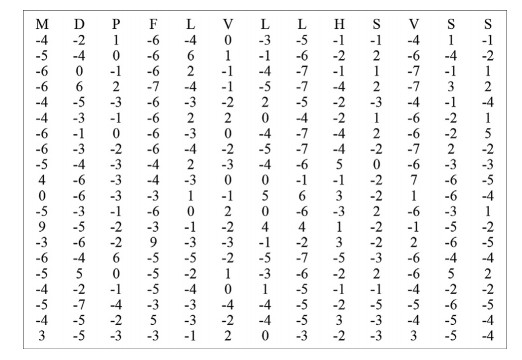
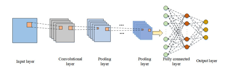
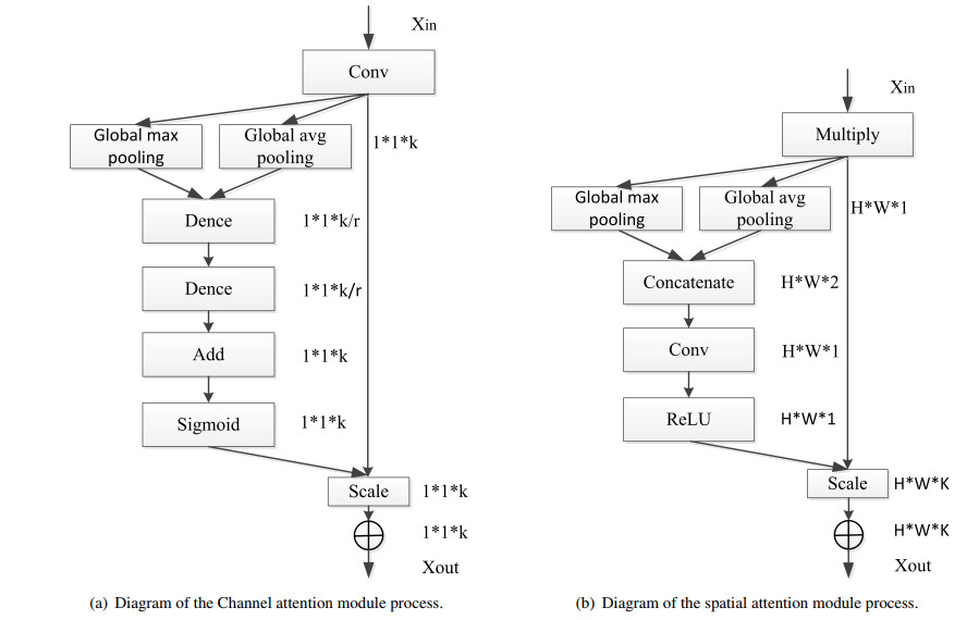
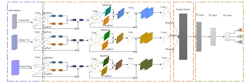
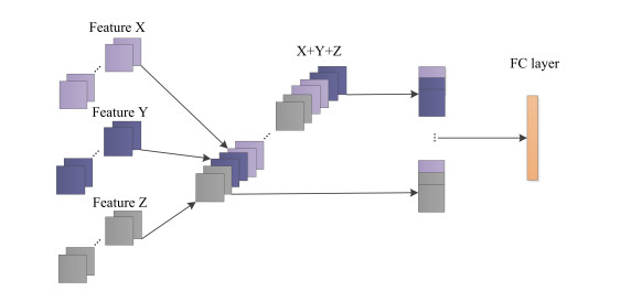
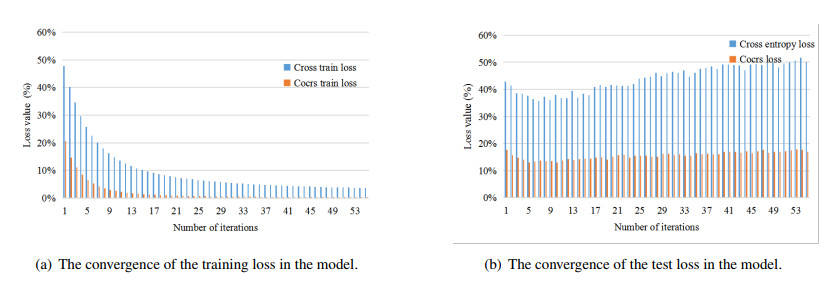
To fully extract the local and long-range information of amino acid sequences and enhance the effective information, this research proposes a secondary structure prediction model of protein based on a multi-scale convolutional attentional neural network. The model uses a multi-channel multi-scale parallel architecture to extract amino acid structure features of different granularity according to the window size. The reconstructed feature maps are obtained via multiple convolutional attention blocks. Then, the reconstructed feature map is fused with the input feature map to obtain the enhanced feature map. Finally, the enhanced feature map is fed to the Softmax classifier for prediction. While the traditional cross-entropy loss cannot effectively solve the problem of non-equilibrium training samples, a modified correlated cross-entropy loss function may alleviate this problem. After numerous comparison and ablation experiments, it is verified that the improved model can indeed effectively extract amino acid sequence feature information, alleviate overfitting, and thus improve the overall prediction accuracy.
Citation: Ying Xu, Jinyong Cheng. Secondary structure prediction of protein based on multi scale convolutional attention neural networks[J]. Mathematical Biosciences and Engineering, 2021, 18(4): 3404-3422. doi: 10.3934/mbe.2021170
To fully extract the local and long-range information of amino acid sequences and enhance the effective information, this research proposes a secondary structure prediction model of protein based on a multi-scale convolutional attentional neural network. The model uses a multi-channel multi-scale parallel architecture to extract amino acid structure features of different granularity according to the window size. The reconstructed feature maps are obtained via multiple convolutional attention blocks. Then, the reconstructed feature map is fused with the input feature map to obtain the enhanced feature map. Finally, the enhanced feature map is fed to the Softmax classifier for prediction. While the traditional cross-entropy loss cannot effectively solve the problem of non-equilibrium training samples, a modified correlated cross-entropy loss function may alleviate this problem. After numerous comparison and ablation experiments, it is verified that the improved model can indeed effectively extract amino acid sequence feature information, alleviate overfitting, and thus improve the overall prediction accuracy.

| [1] |
S. M. Najibi, M. Maadooliat, L. Zhou, J. Z. Huang, X. Gao, Protein structure classification and loop modeling using multiple ramachandran distributions, Comput. Struct. Biotechnol. J., 15 (2017), 243–254. doi: 10.1016/j.csbj.2017.01.011

|
| [2] |
J. Peng, D. Schwartz, J. E. Elias, C. C. Thoreen, D. Cheng, G. Marsischky, et al., A proteomics approach to understanding protein ubiquitination, Nat. Biotechnol., 21 (2003), 921–926. doi: 10.1038/nbt849
|
| [3] |
R. A. Cairns, I. S. Harris, T. W. Mak, Regulation of cancer cell metabolism, Nat. Rev. Cancer, 11 (2011), 85–95. doi: 10.1038/nrc2981
|
| [4] |
X. M. Zhao, R. S. Wang, L. Chen, A. Kazuyuki, Uncovering signal transduction networks from high-throughput data by integer linear programming, Nucleic Acids Res., 36 (2008), e48. doi: 10.1093/nar/gkn145
|
| [5] |
P. Y. Chou, G. D. Fasman, Prediction of protein conformation, Biochemistry, 13 (1974), 222–245. doi: 10.1021/bi00699a002
|
| [6] |
A. Anand, G. Pugalenthi, P. N. Suganthan, Predicting protein structural class by svm with class-wise optimized features and decision probabilities, J. Theor. Biol., 253 (2008), 375–380. doi: 10.1016/j.jtbi.2008.02.031
|
| [7] |
Z. Tang, T. Li, R. Liu, W. Xiong, G. Chen, Improving the performance of $\beta$-turn prediction using predicted shape strings and a two-layer support vector machine model, BMC Bioinf., 12 (2011), 283. doi: 10.1186/1471-2105-12-283
|
| [8] |
S. A. Malekpour, S. Naghizadeh, H. Pezeshk, M. Sadeghi, C. Eslahchi, Protein secondary structure prediction using three neural networks and a segmental semi markov model, Math. Biosci., 217 (2009), 145–150. doi: 10.1016/j.mbs.2008.11.001
|
| [9] |
I. Kurniawan, T. Haryanto, L. S. Hasibuan, M. A. Agmalaro, Combining pssm and physicochemical feature for protein structure prediction with support vector machine, J. Phys. Confer., 835 (2017), 012006. doi: 10.1088/1742-6596/835/1/012006
|
| [10] | Y. Chen, J. Cheng, Y. Liu, P. S. Park, A novel approach of protein secondary structure prediction by svm using pssm combined by sequence features, in Proceedings of SAI Intelligent Systems Conference, Springer, Cham, 2016. |
| [11] | Y. Liu, J. Cheng, Y. Ma, Y. Chen, Protein secondary structure prediction based on two dimensional deep convolutional neural networks, in 2017 3rd IEEE International Conference on Computer and Communications (ICCC), 2017. |
| [12] | M. Alirezaee, Ensemble of neural networks to solve class imbalance problem of protein secondary structure prediction, Int. J. Artif. Intell. Appl., 3 (2012), 9–20. |
| [13] |
B. Zhang, J. Li, L. Qiang, Prediction of 8-state protein secondary structures by a novel deep learning architecture, BMC Bioinf., 19 (2018), 293. doi: 10.1186/s12859-018-2280-5
|
| [14] |
L. J. Mcguffin, K. Bryson, D. T. Jones, The psipred protein structure prediction server, Bioinformatics, 16 (2000), 404–405. doi: 10.1093/bioinformatics/16.4.404
|
| [15] |
Z. Wang, F. Zhao, P. Jian, J. Xu, Protein 8-class secondary structure prediction using conditional neural fields, Proteomics, 11 (2011), 3786–3792. doi: 10.1002/pmic.201100196
|
| [16] | Y. Ma, Y. Liu, J. Cheng, Protein secondary structure prediction based on data partition and semi-random subspace method, Sci. Rep., 8 (2018), 1–10. |
| [17] | A. Yaseen, Y. Li, Template-based c8-scorpion: a protein 8-state secondary structure prediction method using structural information and context-based features, BMC Bioinf., 15 (2014), 1–8. |
| [18] |
R. Heffernan, Y. Yang, K. Paliwal, Y. Zhou, Capturing non-local interactions by long short term memory bidirectional recurrent neural networks for improving prediction of protein secondary structure, backbone angles, contact numbers, and solvent accessibility, Bioinformatics, 33 (2017), 2842–2849 doi: 10.1093/bioinformatics/btx218
|
| [19] |
C. Fang, Y. Shang, X. Dong, Mufold-ss: New deep inception-inside-inception networks for protein secondary structure prediction, Proteins: Struct., Funct., Genet., 86 (2018), 592–598. doi: 10.1002/prot.25487
|
| [20] |
Y. Guo, W. Li, B. Wang, H. Liu, D. Zhou, Deepaclstm: deep asymmetric convolutional long short-term memory neural models for protein secondary structure prediction, BMC Bioinf., 20 (2019), 1–12. doi: 10.1186/s12859-018-2565-8
|
| [21] | I. Drori, I. Dwivedi, P. Shrestha, J. Wan, Y. Wang, Y. He, et al., High quality prediction of protein q8 secondary structure by diverse neural network architectures, in 32nd Conference on Neural Information Processing Systems, Montreal, Canada, 2018. |
| [22] |
C. Fang, Z. Li, D. Xu, Y. Shang, Mufold-ssw: A new web server for predicting protein secondary structures, torsion angles, and turns, Bioinformatics, 36 (2020), 1293–1295. doi: 10.1093/bioinformatics/btz712
|
| [23] |
G. Xu, Q. Wang, J. Ma, Opus-tass: A protein backbone torsion angles and secondary structure predictor based on ensemble neural networks, Bioinformatics, 36 (2020), 5021–5026. doi: 10.1093/bioinformatics/btaa629
|
| [24] |
Y. Zhao, H. Zhang, Y. Liu, Protein secondary structure prediction based on generative confrontation and convolutional neural network, IEEE Access, 8 (2020), 199171–199178. doi: 10.1109/ACCESS.2020.3035208
|
| [25] | W. Kabsch, C. Sander, Dictionary of protein secondary structure: Pattern recognition of hydrogen-bonded and geometrical features, Biopolym.: Orig. Res. Biomol., 22 (1983), 2577–2637. |
| [26] |
G. Wang, R. L. Dunbrack, Pisces: recent improvements to a pdb sequence culling server, Nucleic Acids Res., 33 (2005), W94–W98. doi: 10.1093/nar/gki402
|
| [27] | J. Moult, K. Fidelis, A. Kryshtafovych, A. Tramontano, Critical assessment of methods of protein structure prediction (CASP)-round IX, Proteins: Struct., Funct., Bioinf., 79 (2011), 1–5. |
| [28] | J. Moult, K. Fidelis, A. Kryshtafovych, T. Schwede, A. Tramontano, Critical assessment of methods of protein structure prediction (CASP)-round X, Proteins: Struct., Funct., Bioinf., 82 (2013), 3–9. |
| [29] | J. Moult, K. Fidelis, A. Kryshtafovych, T. Schwede, A. Tramontano, Critical assessment of methods of protein structure prediction (CASP)-round XII, Proteins: Struct., Funct., Bioinf., 86 (2017), 7–15. |
| [30] | W. Kabsch, C. Sander, Dictionary of protein secondary structure: Pattern recognition of hydrogen‐bonded and geometrical features, Biopolymers, 57 (2010), 75–80. |
| [31] |
D. T. Jones, Protein secondary structure prediction based on position-specific scoring matrices., J. Molecul. Biol., 292 (1999), 195–202. doi: 10.1006/jmbi.1999.3091
|
| [32] |
G. Hu, X. Yang, Y. Zhang, M. Wan, Identification of tea leaf diseases by using an improved deep convolutional neural network, Sustainable Comput.: Infor. Syst., 24 (2019), 100353. doi: 10.1016/j.suscom.2019.100353
|
| [33] | N. Abramson, D. J. Braverman, G. S. Sebestyen, Pattern recognition and machine learning, Publ. Am. Stat. Assoc., 103 (2006), 886–887. |
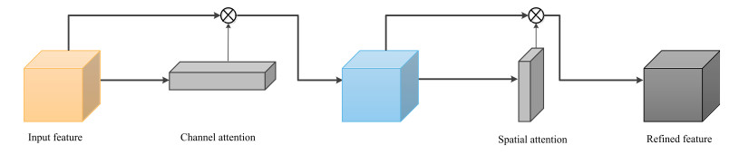
| [34] | S. Woo, J. Park, J. Y. Lee, I. S. Kweon, Cbam: Convolutional block attention module, in Computer Vision – ECCV 2018. Lecture Notes in Computer Science, Springer, Cham, 2018. |
| [35] | S. Wang, J. Peng, J. Ma, J. Xu, Protein secondary structure prediction using deep convolutional neural fields, Sci. Rep., 6 (2016), 886–887. |
| [36] |
A. Drozdetskiy, C. Cole, J. Procter, G. J. Barton, JPred4: a protein secondary structure prediction server, Nucleic Acids Res., 43 (2015), W389–W394. doi: 10.1093/nar/gkv332
|
Figures(10) / Tables(5)

Ying Xu, Jinyong Cheng. Secondary structure prediction of protein based on multi scale convolutional attention neural networks[J]. Mathematical Biosciences and Engineering, 2021, 18(4): 3404-3422. doi: 10.3934/mbe.2021170


 DownLoad: