A hybrid model for forecasting of particulate matter concentrations based on multiscale characterization and machine learning techniques

Syed Ahsin Ali Shah; Wajid Aziz; Majid Almaraashi; Malik Sajjad Ahmed Nadeem; Nazneen Habib; Seong-O Shim; Syed Ahsin Ali Shah; Wajid Aziz; Majid Almaraashi; Malik Sajjad Ahmed Nadeem; Nazneen Habib; Seong-O Shim

doi:10.3934/mbe.2021104

Mathematical Biosciences and Engineering

2021, Volume 18, Issue 3: 1992-2009. doi: 10.3934/mbe.2021104

Previous Article Next Article

Research article

A hybrid model for forecasting of particulate matter concentrations based on multiscale characterization and machine learning techniques

1.
Department of Computer Science & IT, University of Azad Jammu and Kashmir, King Abdullah Campus, Muzaffarabad 13100, AJK, Pakistan
2.
College of Computer Science & Engineering, University of Jeddah, Jeddah 23890, Saudi Arabia
3.
Department of Sociology & Rural Development, University of Azad Jammu Kashmir, Muzaffarabad 13100, AJK, Pakistan

Received: 06 December 2020 Accepted: 04 February 2021 Published: 02 March 2021

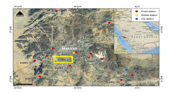
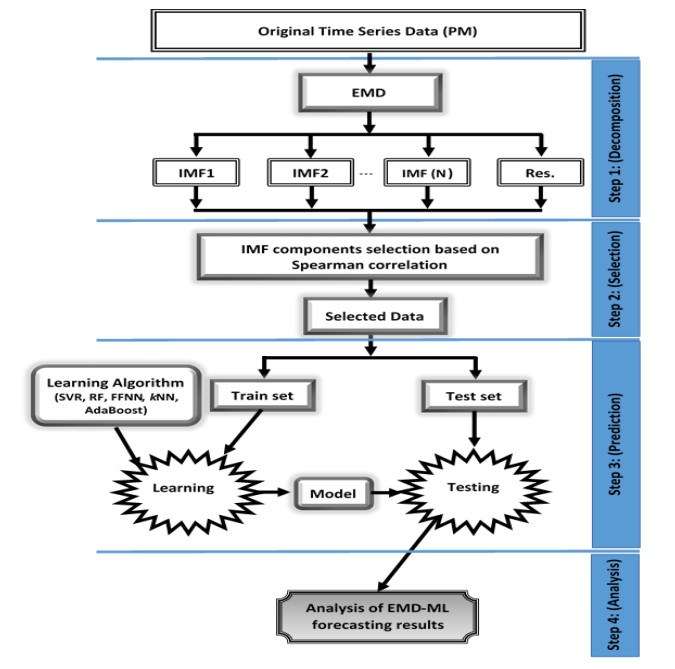
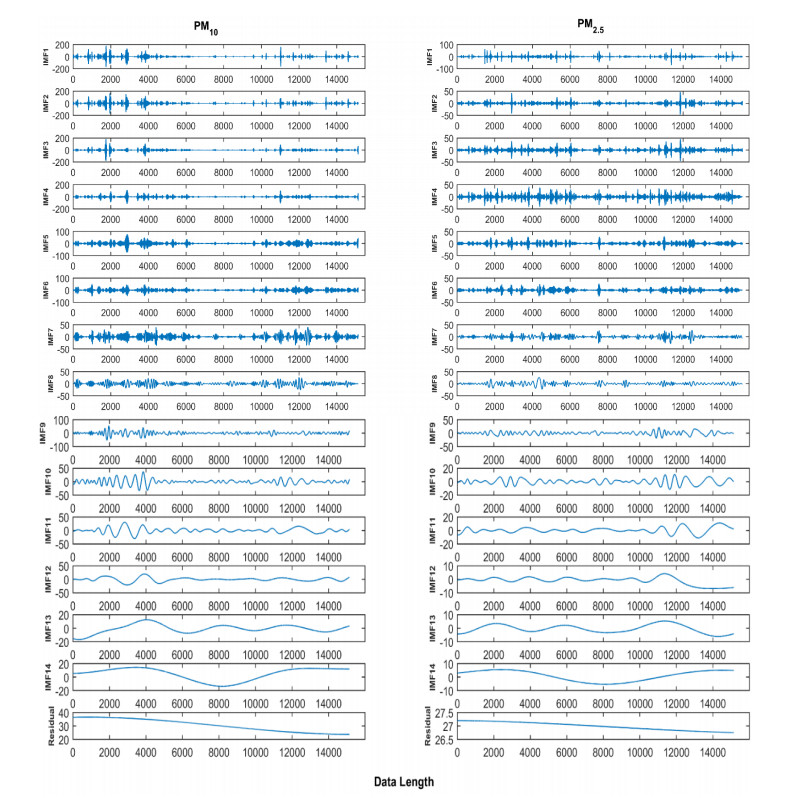
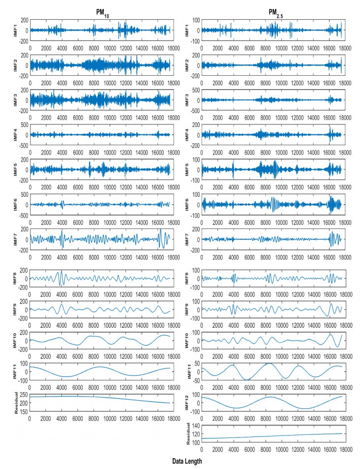
Accurate prediction of particulate matter (PM) using time series data is a challenging task. The recent advancements in sensor technology, computing devices, nonlinear computational tools, and machine learning (ML) approaches provide new opportunities for robust prediction of PM concentrations. In this study, we develop a hybrid model for forecasting PM₁₀ and PM_2.5 based on the multiscale characterization and ML techniques. At first, we use the empirical mode decomposition (EMD) algorithm for multiscale characterization of PM₁₀ and PM_2.5 by decomposing the original time series into numerous intrinsic mode functions (IMFs). Different individual ML algorithms such as random forest (RF), support vector regressor (SVR), k-nearest neighbors (kNN), feed forward neural network (FFNN), and AdaBoost are then used to develop EMD-ML models. The air quality time series data from Masfalah air station Makkah, Saudi Arabia are utilized for validating the EMD-ML models, and results are compared with non-hybrid ML models. The PMs (PM₁₀ and PM_2.5) concentrations data of Dehli, India are also utilized for validating the EMD-ML models. The performance of each model is evaluated using root mean square error (RMSE) and mean absolute error (MAE). The average bias in the predictive model is estimated using mean bias error (MBE). Obtained results reveal that EMD-FFNN model provides the lowest error rate for both PM₁₀ (RMSE = 12.25 and MAE = 7.43) and PM_2.5 (RMSE = 4.81 and MAE = 3.02) using Misfalah, Makkah data whereas EMD-kNN model provides the lowest error rate for PM₁₀ (RMSE = 20.56 and MAE = 12.87) and EMD-AdaBoost provides the lowest error rate for PM_2.5 (RMSE = 15.29 and MAE = 9.45) using Dehli, India data. The findings also reveal that EMD-ML models can be effectively used in forecasting PM mass concentrations and to develop rapid air quality warning systems.
- empirical mode decomposition,
- forecasting,
- hybrid forecasting model,
- machine learning algorithms,
- particulate matter
Citation: Syed Ahsin Ali Shah, Wajid Aziz, Majid Almaraashi, Malik Sajjad Ahmed Nadeem, Nazneen Habib, Seong-O Shim. A hybrid model for forecasting of particulate matter concentrations based on multiscale characterization and machine learning techniques[J]. Mathematical Biosciences and Engineering, 2021, 18(3): 1992-2009. doi: 10.3934/mbe.2021104

Related Papers:

Abstract

Accurate prediction of particulate matter (PM) using time series data is a challenging task. The recent advancements in sensor technology, computing devices, nonlinear computational tools, and machine learning (ML) approaches provide new opportunities for robust prediction of PM concentrations. In this study, we develop a hybrid model for forecasting PM₁₀ and PM_2.5 based on the multiscale characterization and ML techniques. At first, we use the empirical mode decomposition (EMD) algorithm for multiscale characterization of PM₁₀ and PM_2.5 by decomposing the original time series into numerous intrinsic mode functions (IMFs). Different individual ML algorithms such as random forest (RF), support vector regressor (SVR), k-nearest neighbors (kNN), feed forward neural network (FFNN), and AdaBoost are then used to develop EMD-ML models. The air quality time series data from Masfalah air station Makkah, Saudi Arabia are utilized for validating the EMD-ML models, and results are compared with non-hybrid ML models. The PMs (PM₁₀ and PM_2.5) concentrations data of Dehli, India are also utilized for validating the EMD-ML models. The performance of each model is evaluated using root mean square error (RMSE) and mean absolute error (MAE). The average bias in the predictive model is estimated using mean bias error (MBE). Obtained results reveal that EMD-FFNN model provides the lowest error rate for both PM₁₀ (RMSE = 12.25 and MAE = 7.43) and PM_2.5 (RMSE = 4.81 and MAE = 3.02) using Misfalah, Makkah data whereas EMD-kNN model provides the lowest error rate for PM₁₀ (RMSE = 20.56 and MAE = 12.87) and EMD-AdaBoost provides the lowest error rate for PM_2.5 (RMSE = 15.29 and MAE = 9.45) using Dehli, India data. The findings also reveal that EMD-ML models can be effectively used in forecasting PM mass concentrations and to develop rapid air quality warning systems.

References

[1]	B. Chen, H. Kan, Air pollution and population health: A global challenge, Environ. Health Prev. Med., 13 (2008), 94-101. doi: 10.1007/s12199-007-0018-5
[2]	R. Habre, B. Coull, E. Moshier, J. Godbold, A. Grunin, A. Nath, et al., Sources of indoor air pollution in New York city residences of asthmatic children, J. Expo. Sci. Environ. Epidemiol., 24 (2014), 269-278. doi: 10.1038/jes.2013.74
[3]	D. L. Robinson, Air pollution in Australia: Review of costs sources and potential solutions, Health Promot. J. Austr., 16 (2005), 213-220. doi: 10.1071/HE05213
[4]	H. S. Rumana, R. C. Sharma, V. Beniwal, A. K. Sharma, A retrospective approach to assess human health risks associated with growing air pollution in urbanized area of Thar Desert, western Rajasthan, India, J. Environ. Health Sci. Eng., 12 (2014), 23. doi: 10.1186/2052-336X-12-23
[5]	S. Yamamoto, R. Phalkey, A. Malik, A systematic review of air pollution as a risk factor for cardiovascular disease in South Asia: Limited evidence from India and Pakistan, Int. J. Hyg. Environ. Health, 217 (2014), 133-144. doi: 10.1016/j.ijheh.2013.08.003
[6]	W. Zhang, C. N. Qian, Y. X. Zeng, Air pollution: A smoking gun for cancer, Chin. J. Cancer, 33 (2014), 173.
[7]	H. Kan, B. Chen, N. Zhao, S. J. London, G. Song, G. Chen, et al., Part 1: A time-series study of ambient air pollution and daily mortality in Shanghai, China, Res. Rep. Health. Eff. Inst., 154 (2010), 17-78.
[8]	K. Vermaelen, G. Brusselle, Exposing a deadly alliance: Novel insights into the biological links between COPD and lung cancer, Pulm. Pharmacol. Ther., 26 (2013), 544-554. doi: 10.1016/j.pupt.2013.05.003
[9]	WHO., Burden of disease from the joint effects of household and ambient air pollution for 2016, Soc. Environ. Determ. Health Dep.: Geneva, Switzerland, 7 (2018).
[10]	C A. Pope Ⅲ, D. W. Dockery, Health effects of fine particulate air pollution: Lines that connect, J. Air Waste Manag. Assoc., 56 (2006), 709-742. doi: 10.1080/10473289.2006.10464485
[11]	R. Shad, M. S. Mesgari, A. Shad, Predicting air pollution using fuzzy genetic linear membership kriging in GIS, Comput. Environ. Urban Syst., 33 (2009), 472-481. doi: 10.1016/j.compenvurbsys.2009.10.004
[12]	J. G. Titus, Greenhouse Effect, Sea Level Rise, and Barrier Islands: Case Study of Long Beach Island, New Jersey, 1990.
[13]	S. A. A. Shah, W. Aziz, M. S. A. Nadeem, M. Almaraashi, S. O. Shim, T. M. Habeebullah, A novel phase space reconstruction (PSR) based predictive algorithm to forecast atmospheric particulate matter concentration, Sci. Program., 2019.
[14]	J. Zhu, P. Wu, H. Chen, L. Zhou, Z. Tao, A hybrid forecasting approach to air quality time series based on endpoint condition and combined forecasting model, Int. J. Eviron. Res. Pub. Health, 15 (2018), 1941. doi: 10.3390/ijerph15091941
[15]	A. B. Chelani, S. Devotta, Air quality forecasting using a hybrid autoregressive and nonlinear model, Atmos. Environ., 40 (2006), 1774-1780. doi: 10.1016/j.atmosenv.2005.11.019
[16]	N. E. Huang, Z. Shen, S. R. Long, M. C. Wu, H. H. Shih, Q. Zheng, et al., The empirical mode decomposition and the Hilbert spectrum for nonlinear and non-stationary time series analysis, Proc. Math. Phys. Eng. Sci., 454 (1998), 903-995. doi: 10.1098/rspa.1998.0193
[17]	Q. Chen, D. Wen, X. Li, D. Chen, H. Lv, J. Zhang, et al., Empirical mode decomposition based long short-term memory neural network forecasting model for the short-term metro passenger flow, PloS one, 14 (2019), 222365.
[18]	O. K. Cura, S. K. Atli, H. S. Türe, A. Akan, Epileptic seizure classifications using empirical mode decomposition and its derivative, Bio. Med. Eng. OnLine, 19 (2020), 1-22. doi: 10.1186/s12938-019-0745-z
[19]	J. Song, J. Wang, H. Lu, A novel combined model based on advanced optimization algorithm for short-term wind speed forecasting, Appl. Energy, 215 (2018), 643-658. doi: 10.1016/j.apenergy.2018.02.070
[20]	J. N. Wang, J. Du, C. Jiang, K. K. Lai, Chinese currency exchange rates forecasting with EMD-based neural network, Complexity, 2019.
[21]	W. Xu, H. Hu, W. Yang, Energy time series forecasting based on empirical mode decomposition and FRBF-AR model, IEEE Access, 7 (2019), 36540-36548. doi: 10.1109/ACCESS.2019.2902510
[22]	L. Yu, Z. Wang, L. Tang, A decomposition‑ensemble model with data-characteristic-driven reconstruction for crude oil price forecasting, Appl. Energy, 156 (2015), 251-267. doi: 10.1016/j.apenergy.2015.07.025
[23]	X. Zhang, J. Wang, A novel decomposition-ensemble model for forecasting short-term load-time series with multiple seasonal patterns, Appl. Soft Comput., 65 (2018), 478-494. doi: 10.1016/j.asoc.2018.01.017
[24]	Z. Guan, Z. Liao, K. Li, P. Chen, A precise diagnosis method of structural faults of rotating machinery based on combination of empirical mode decomposition, sample entropy and deep belief network, Sensors, 19 (2019), 591. doi: 10.3390/s19030591
[25]	X. B. Jin, N. X. Yang, X. Y. Wang, Y. T. Bai, T. L. Su, J. L. Kong, Hybrid deep learning predictor for smart agriculture sensing based on empirical mode decomposition and gated recurrent unit group model, Sensors, 20(2020), 1334. doi: 10.3390/s20051334
[26]	O. Vargas-Lopez, J. P. Amezquita-Sanchez, J. J. De-Santiago-Perez, J. R. Rivera-Guillen, M. Valtierra-Rodriguez, M. Toledano-Ayala, et al., A new methodology based on EMD and nonlinear measurements for sudden cardiac death detection, Sensors, 20 (2020), 9.
[27]	S. Zhu, X. Lian, H. Liu, J. Hu, Y. Wang, J. Che, Daily air quality index forecasting with hybrid models: A case in China, Environ. Pollut., 231 (2017), 1232-1244. doi: 10.1016/j.envpol.2017.08.069
[28]	K. Pholsena, L. Pan, Z. Zheng, Mode decomposition based deep learning model for multi-section traffic prediction, World Wide Web, 23 (2020), 2513-2527. doi: 10.1007/s11280-020-00791-1
[29]	Q. Zhou, H. Jiang, J. Wang, J. Zhou, A hybrid model for PM2.5 forecasting based on ensemble empirical mode decomposition and a general regression neural network, Sci. Total Environ., 496 (2014), 264-274. doi: 10.1016/j.scitotenv.2014.07.051
[30]	M. Niu, Y. Wang, S. Sun, Y. Li, A novel hybrid decomposition-and-ensemble model based on CEEMD and GWO for short-term PM2.5 concentration forecasting, Atmos. Environ., 134 (2016), 168-180. doi: 10.1016/j.atmosenv.2016.03.056
[31]	S. Munir, T. M. Habeebullah, A. M. Mohammed, E. A. Morsy, M. Rehan, K. Ali, Analysing PM2.5 and its association with PM10 and meteorology in the arid climate of Makkah, Saudi Arabia, Aerosol Air Qual. Res., 17 (2016), 453-464.
[32]	T. M. Habeebullah, S. Munir, E. A. Morsy, A. M. Mohammed, Spatial and temporal analysis of air pollution in Makkah, the Kingdom of Saudi Arabia, 2010 5^th Int. Conf. Environ. Sci. Tech., IPCBEE, 2010, 65-70.
[33]	P. Kline, The new psychometrics: Science, psychology and measurement, Psychol. Press, 1998.
[34]	A. Olinsky, S. Chen, L. Harlow, The comparative efficacy of imputation methods for missing data in structural equation modeling, Eur. J. Oper. Res., 151 (2003), 53-79. doi: 10.1016/S0377-2217(02)00578-7
[35]	Vopani, Air Quality Data in India (2015-2020), Version 12, Available from https://www.kaggle.com/rohanrao/air-quality-data-in-india/version/12.
[36]	G. P. Zhang, Neural networks for time-series forecasting, Springer Berlin Heidelberg, 2012.
[37]	Y. Freund, R. E. Schapire, A short introduction to boosting, J. Jpn. Soc. Artif. Intell., 14 (1999), 771-780.
[38]	L. Breiman, Random forests, Mach. Learn., 45 (2001), 5-32. doi: 10.1023/A:1010933404324
[39]	E. Fix, J. Hodges, Discriminatory analysis: Nonparametric discrimination consistency properties, USAF School Avi. Med. Project, (1952), 21-49.
[40]	T. Bailey, A note on distance-weighted k-nearest neighbor rules, IEEE Trans. Syst. Man, Cybernet., 8 (1978), 311-313. doi: 10.1109/TSMC.1978.4309958
[41]	H. Drucker, C. J. Burges, L. Kaufman, A. J. Smola, V. Vapnik, Support vector regression machines, Proc. Adv. Neural Inf. Process. Syst., (1997), 155-161.

Reader Comments

Your name:*

Email:*
© 2021 the Author(s), licensee AIMS Press. This is an open access article distributed under the terms of the Creative Commons Attribution License (http://creativecommons.org/licenses/by/4.0)