This research investigates an approximate solution to the nonlinear temporal-fractional Allen-Cahn equation (A-CE), a fundamental model for the dynamics of phase separation in binary alloys and pattern formation in physical systems. The conventional integer-order A-CE is extended to a fractional-order model employing the Caputo fractional derivative to capture long-range dependencies and memory effects. The modified generalized Mittag-Leffler function method (MGMLFM) and the Temimi-Ansari method (TAM) are employed as two analytical methods to achieve the study's goal. These methods provide a rapidly convergent solution to the known exact solution. Additionally, a comparison between the error analysis of these methods and the results obtained from other methods found in the literature, such as the Elzaki iterative transform method (EITM), homotopy perturbation method (HPM), new iterative transform method (NITM), Laplace residual power series method (LRPSM), and homotopy analysis method (HAM), to verify the accuracy of both methods. The simulation results are displayed in 2D and 3D plots and data tables. The outcomes confirm that the approximate solution when $ \alpha\rightarrow 1 $ converges very closely with the exact solution. The absolute errors are competitive with, and in many tested cases smaller than, those of other published methods; however, the comparison is not uniformly favorable, and the relative accuracy depends on the specific space–time point and fractional order. The numerical results indicate that the relative accuracy of the MGMLFM and the HAM varies across the considered space-time points and fractional orders. The proposed framework establishes both the MGMLFM and the TAM as powerful tools to analyze complex fractional-order nonlinear systems that emerge in materials science and engineering.
Citation: Hegagi Mohamed Ali, Wedad Albalawi. Theoretical and computational aspects for the nonlinear time-fractional Allen-Cahn model using two efficient approaches[J]. AIMS Mathematics, 2026, 11(11): 37289-37310. doi: 10.3934/math.20261442
This research investigates an approximate solution to the nonlinear temporal-fractional Allen-Cahn equation (A-CE), a fundamental model for the dynamics of phase separation in binary alloys and pattern formation in physical systems. The conventional integer-order A-CE is extended to a fractional-order model employing the Caputo fractional derivative to capture long-range dependencies and memory effects. The modified generalized Mittag-Leffler function method (MGMLFM) and the Temimi-Ansari method (TAM) are employed as two analytical methods to achieve the study's goal. These methods provide a rapidly convergent solution to the known exact solution. Additionally, a comparison between the error analysis of these methods and the results obtained from other methods found in the literature, such as the Elzaki iterative transform method (EITM), homotopy perturbation method (HPM), new iterative transform method (NITM), Laplace residual power series method (LRPSM), and homotopy analysis method (HAM), to verify the accuracy of both methods. The simulation results are displayed in 2D and 3D plots and data tables. The outcomes confirm that the approximate solution when $ \alpha\rightarrow 1 $ converges very closely with the exact solution. The absolute errors are competitive with, and in many tested cases smaller than, those of other published methods; however, the comparison is not uniformly favorable, and the relative accuracy depends on the specific space–time point and fractional order. The numerical results indicate that the relative accuracy of the MGMLFM and the HAM varies across the considered space-time points and fractional orders. The proposed framework establishes both the MGMLFM and the TAM as powerful tools to analyze complex fractional-order nonlinear systems that emerge in materials science and engineering.

| [1] |
H. Tariq, G. Akram, New traveling wave exact and approximate solutions for the nonlinear Cahn-Allen equation: evolution of a nonconserved quantity, Nonlinear Dyn., 88 (2017), 581–594. https://doi.org/10.1007/s11071-016-3262-7 doi: 10.1007/s11071-016-3262-7
|
| [2] |
H. G. Lee, Y. Hwang, Y. Nam, S. Kim, J. Kim, Benchmark problems for physics-informed neural networks: the Allen-Cahn equation, AIMS Math., 10 (2025), 7319–7338. https://doi.org/10.3934/math.2025335 doi: 10.3934/math.2025335
|
| [3] |
M. M. A. Khater, A. R. Seadawy, D. Lu, Elliptic and solitary wave solutions for Bogoyavlenskii equations system, couple Boiti-Leon-Pempinelli equations system and time-fractional Cahn-Allen equation, Results Phys., 7 (2017), 2325–2333. https://doi.org/10.1016/j.rinp.2017.06.049 doi: 10.1016/j.rinp.2017.06.049
|
| [4] |
G. Hariharan, K. Kannan, Haar wavelet method for solving Cahn-Allen equation, Appl. Math. Sci., 3 (2009), 2523–2533. |
| [5] |
L. Ali, R. Shah, W. Weera, Fractional view analysis of Cahn–Allen equations by new iterative transform method, Fractal Fract., 6 (2022), 293. https://doi.org/10.3390/fractalfract6060293 doi: 10.3390/fractalfract6060293
|
| [6] |
I. Khan, R. Nawaz, A. H. Ali, A. Akgul, S. A. Lone, Comparative analysis of the fractional order Cahn-Allen equation, Partial Differ. Equ. Appl. Math., 8 (2023), 100576. https://doi.org/10.1016/j.padiff.2023.100576 doi: 10.1016/j.padiff.2023.100576
|
| [7] |
A. Esen, N. M. Yagmurlu, O. Tasbozan, Approximate analytical solution to time-fractional damped Burger and Cahn-Allen equations, Appl. Math. Inf. Sci., 7 (2013), 1951–1956. https://doi.org/10.12785/amis/070533 doi: 10.12785/amis/070533
|
| [8] |
H. Kim, Q. Jin, X. Wu, S. Kwak, Z. Li, J. Kim, An adaptive numerical method for solving the Allen–Cahn equation on curved surfaces, J. Comput. Appl. Math., 486 (2026), 117702. https://doi.org/10.1016/j.cam.2026.117702 doi: 10.1016/j.cam.2026.117702
|
| [9] |
H. Kim, J. Ma, H. Shin, J. Kim, An efficient and accurate adaptive time-stepping method for the Allen–Cahn equation, Comput. Math. Appl., 212 (2026), 62–77. https://doi.org/10.1016/j.camwa.2026.03.014 doi: 10.1016/j.camwa.2026.03.014
|
| [10] |
H. KIM, Numerical dynamics for the Allen–Cahn equation with variable mobility on curved surfaces, J. Korean Soc. Ind. Appl. Math., 29 (2025), 360–376. |
| [11] |
A. A. Kilbas, H. M. Srivastava, J. J. Trujillo, Theory and applications of fractional differential equations, Vol. 204, Amsterdam: Elsevier, 2006. https://doi.org/10.1016/S0304-0208(06)X8001-5 |
| [12] |
H. M. Ali, K. S. Nisar, W. R. Alharbi, M. Zakarya, Efficient approximate analytical technique to solve nonlinear coupled Jaulent–Miodek system within a time-fractional order, AIMS Math., 9 (2024), 5671–5685. https://doi.org/10.3934/math.2024274 doi: 10.3934/math.2024274
|
| [13] |
P. Agarwal, L. Vázquez Martínez, E. K. Lenzi, Recent trends in fractional calculus and its applications, Elsevier, 2024. https://doi.org/10.1016/C2022-0-00393-7 |
| [14] |
D. Baleanu, R. P. Agarwal, uFractional calculus in the sky, Adv. Diff. Equ., 2021 (2021), 117. https://doi.org/10.1186/s13662-021-03270-7 doi: 10.1186/s13662-021-03270-7
|
| [15] |
A. A. M. Arafa, S. Z. Rida, H. Mohamed, Homotopy analysis method for solving biological population model, Commun. Theor. Phys., 56 (2011), 797–800. https://doi.org/10.1088/0253-6102/56/5/01 doi: 10.1088/0253-6102/56/5/01
|
| [16] |
D. D. Ganji, A. Sadighi, Application of homotopy-perturbation and variational iteration methods to nonlinear heat transfer and porous media equations, J. Comput. Appl. Math., 207 (2007), 24–34. https://doi.org/10.1016/j.cam.2006.07.030 doi: 10.1016/j.cam.2006.07.030
|
| [17] |
N. Iqbal, M. T. Chughtai, R. Ullah, Fractional study of the non-linear Burgers equations via a semi-analytical technique, Fractal Fract., 7 (2023), 103. https://doi.org/10.3390/fractalfract7020103 doi: 10.3390/fractalfract7020103
|
| [18] |
M. Abbaszadeh, M. Dehghan, A reduced order finite difference method for solving space-fractional reaction-diffusion systems: the Gray-Scott model, Eur. Phys. J. Plus, 134 (2019), 620. https://doi.org/10.1140/epjp/i2019-12951-0 doi: 10.1140/epjp/i2019-12951-0
|
| [19] |
S. Tuluce Demiray, H. Bulut, F. B. M. Belgacem, Sumudu transform method for analytical solutions of fractional type ordinary differential equations, Math. Probl. Eng., 2015 (2015), 131690. https://doi.org/10.1155/2015/131690 doi: 10.1155/2015/131690
|
| [20] |
D. B. Dhaigude, G. A. Birajdar, Numerical solution of fractional partial differential equations by discrete Adomian decomposition method, Adv. Appl. Math. Mech., 6 (2014), 107–119. https://doi.org/10.4208/aamm.12-m12105 doi: 10.4208/aamm.12-m12105
|
| [21] |
O. P. Yadav, R. Jiwari, A finite element approach for analysis and computational modelling of coupled reaction diffusion models, Numer. Meth. Partial Diff. Equ., 35 (2019), 830–850. https://doi.org/10.1002/num.22328 doi: 10.1002/num.22328
|
| [22] |
S. Javeed, D. Baleanu, A. Waheed, M. S. Khan, H. Affan, Analysis of homotopy perturbation method for solving fractional order differential equations, Mathematics, 7 (2019), 40. https://doi.org/10.3390/math7010040 doi: 10.3390/math7010040
|
| [23] |
H. M. Ali, Analytical investigation of the fractional nonlinear shallow-water model, J. Appl. Math. Comput., 70 (2024), 5497–5514. https://doi.org/10.1007/s12190-024-02172-7 doi: 10.1007/s12190-024-02172-7
|
| [24] |
A. A. M. Arafa, S. Z. Rida, A. A. Mohammadein, H. M. Ali, Solving nonlinear fractional differential equation by generalized Mittag-Leffler function method, Commun. Theor. Phys., 59 (2013), 661–663. https://doi.org/10.1088/0253-6102/59/6/01 doi: 10.1088/0253-6102/59/6/01
|
| [25] |
J. Singh, D. Kumar, D. Baleanu, S. Rathore, An efficient numerical algorithm for the fractional Drinfeld-Sokolov-Wilson equation, Appl. Math. Comput., 335 (2018), 12–24. https://doi.org/10.1016/j.amc.2018.04.025 doi: 10.1016/j.amc.2018.04.025
|
| [26] |
H. Temimi, A. R. Ansari, A semi-analytical iterative technique for solving nonlinear problems, Comput. Math. Appl., 61 (2011), 203–210. https://doi.org/10.1016/j.camwa.2010.10.042 doi: 10.1016/j.camwa.2010.10.042
|
| [27] |
I. Podlubny, Fractional differential equations, Mathematics in Sciences and Engineering, Vol. 198, San Diego: Academic Press, 1999. https://doi.org/10.1016/S0076-5392(99)X8001-5 |
| [28] |
D. Baleanu, K. Diethelm, E. Scalas, J. J. Trujillo, Fractional calculus: models and numerical methods, Series on Complexity, Nonlinearity and Chaos, Vol. 3, Singapore, New Jersey, London and Hong Kong: World Scientific Publishing Company, 2012. https://doi.org/10.1142/8180 |
| [29] |
H. Thabet, S. Kendre, J. Peters, Travelling wave solutions for fractional Korteweg-de Vries equations via an approximate-analytical method, AIMS Math., 4 (2019), 1203–1222. https://doi.org/10.3934/math.2019.4.1203 doi: 10.3934/math.2019.4.1203
|
| [30] |
A. Ghorbani, Beyond Adomian polynomials: He polynomials, Chaos Soliton. Fract., 39 (2009), 1486–1492. https://doi.org/10.1016/j.chaos.2007.06.034 doi: 10.1016/j.chaos.2007.06.034
|
Figures(6) / Tables(5)

Hegagi Mohamed Ali, Wedad Albalawi. Theoretical and computational aspects for the nonlinear time-fractional Allen-Cahn model using two efficient approaches[J]. AIMS Mathematics, 2026, 11(11): 37289-37310. doi: 10.3934/math.20261442

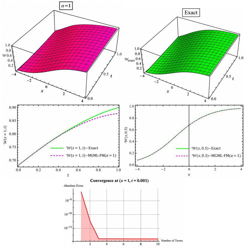
The 3D and 2D behavior of the MGMLFM approximate solution (four-term fractional series) when $ \alpha = 1 $ and the exact solution of $ \mathscr{W}(x, t) $ in Problem (1.1). The 2D plot at $ t = 0.5 $ with a spatial range of $ x \in [-4, 4] $ and at $ x = 1 $ with a temporal range of $ t \in [0, 1] $
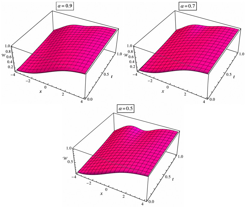
Behavior of the MGMLFM approximate solution (four-term fractional series) for $ \mathscr{W}(x, t) $ in Problem (1.1) at different values of $ \alpha = 0.9, 0.7, 0.5 $ with a spatial range of $ x \in [-4, 4] $ and a temporal range of $ t \in [0, 1] $
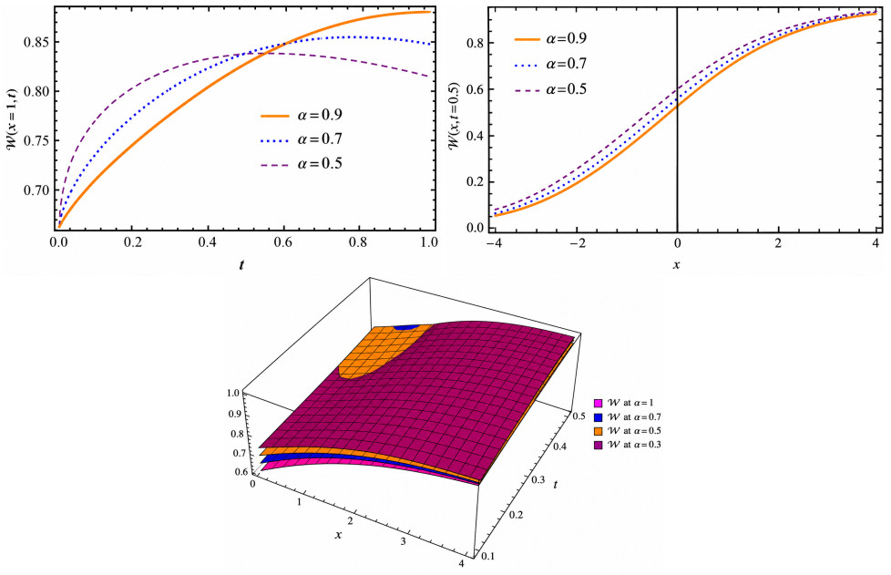
The 2D and 3D behavior of the MGMLFM approximate solution (four-term fractional series) for $ \mathscr{W}(x, t) $ in Problem (1.1) at various values of $ \alpha = 0.9, 0.7, 0.5 $ with a spatial range of $ x \in [-4, 4] $ and a temporal range of $ t \in [0, 1] $
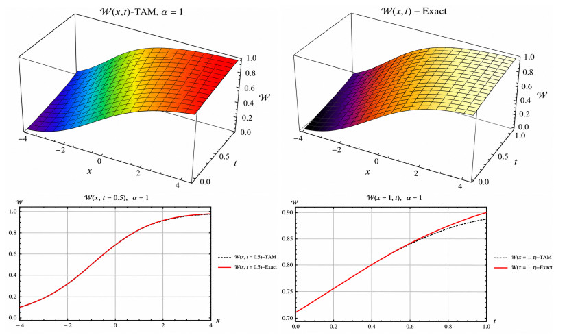
The 3D and 2D behavior of the TAM approximate solution (4 iterations) when $ \alpha = 1 $ and the exact solution of $ \mathscr{W}(x, t) $ in Problem (1.1). The 2D plot at $ t = 0.5 $ with a spatial range of $ x \in [-4, 4] $ and at $ x = 1 $ with a temporal range of $ t \in [0, 1] $
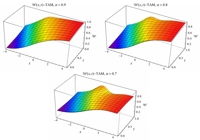
The behavior of the TAM approximate solution (4 iterations) for $ \mathscr{W}(x, t) $ in Problem (1.1) at $ \alpha = 0.9, 0.8, 0.7 $ with a spatial range of $ x \in [-4, 4] $ and a temporal range of $ t \in [0, 1] $
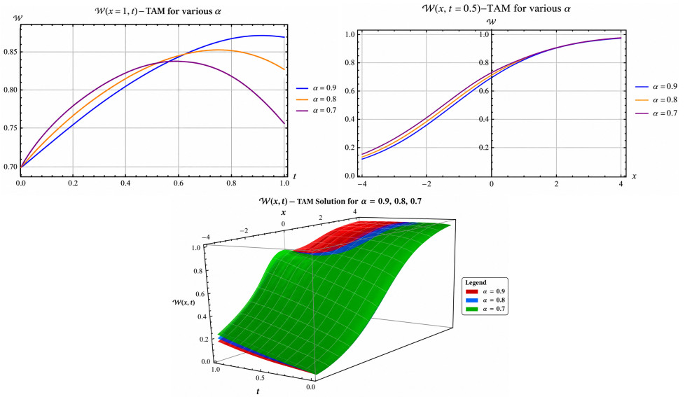
The 2D and 3D behavior of the TAM approximate solution (4 iterations) for $ \mathscr{W}(x, t) $ in Problem (1.1) at various values of $ \alpha = 0.9, 0.8, 0.7 $ with a spatial range of $ x \in [-4, 4] $ and a temporal range of $ t \in [0, 1] $. The 2D plot at $ t = 0.5 $ with a spatial range of $ x \in [-4, 4] $ and at $ x = 1 $ with a temporal range of $ t \in [0, 1] $




 DownLoad: