This paper presents a mathematical model for viral marketing diffusion on complex networks. The model considers four compartmental states: targets, who are initially unaware of the advertised product; spreading clients, who disseminate information and are customers of the product; spreading nonclients, who disseminate information without being customers; and inactive individuals, who are aware of the product but do not participate in its dissemination.
The proposed framework builds on established node-based mean-field approaches to spreading processes on complex networks. Specifically, deterministic equations are obtained through a first-order mean-field approximation to an interacting continuous-time stochastic process on the contact network. Consequently, the resulting node-level probabilities approximate the marginal state probabilities of the underlying stochastic process.
The distinguishing feature of the model is the explicit separation between spreading clients and spreading nonclients, allowing the diffusion of advertising information to be studied while retaining information about the customer status of the individuals involved.
The model incorporates the topology of the contact network and allows heterogeneous transition parameters. We analyze its diffusion dynamics, derive invasion thresholds for the network model and its homogeneous reduction, and investigate the accuracy of the mean-field approximation through comparisons with stochastic Monte Carlo simulations.
The proposed approach thus provides a marketing-oriented application of established network diffusion modeling techniques rather than a new general mathematical framework for individual-based spreading processes.
Citation: Angel Martin del Rey, Jose D. Hernandez Guillen. An individual-based mean-field network model for viral marketing diffusion[J]. AIMS Mathematics, 2026, 11(11): 36771-36805. doi: 10.3934/math.20261422
This paper presents a mathematical model for viral marketing diffusion on complex networks. The model considers four compartmental states: targets, who are initially unaware of the advertised product; spreading clients, who disseminate information and are customers of the product; spreading nonclients, who disseminate information without being customers; and inactive individuals, who are aware of the product but do not participate in its dissemination.
The proposed framework builds on established node-based mean-field approaches to spreading processes on complex networks. Specifically, deterministic equations are obtained through a first-order mean-field approximation to an interacting continuous-time stochastic process on the contact network. Consequently, the resulting node-level probabilities approximate the marginal state probabilities of the underlying stochastic process.
The distinguishing feature of the model is the explicit separation between spreading clients and spreading nonclients, allowing the diffusion of advertising information to be studied while retaining information about the customer status of the individuals involved.
The model incorporates the topology of the contact network and allows heterogeneous transition parameters. We analyze its diffusion dynamics, derive invasion thresholds for the network model and its homogeneous reduction, and investigate the accuracy of the mean-field approximation through comparisons with stochastic Monte Carlo simulations.
The proposed approach thus provides a marketing-oriented application of established network diffusion modeling techniques rather than a new general mathematical framework for individual-based spreading processes.

| [1] |
M. T. Ewing, D. B. Stewart, D. R. Mather, J. D. Newton, How contagious is your viral marketing campaign? A mathematical model for assessing campaign performance, J. Advert. Res., 54 (2014), 205–216. https://doi.org/10.2501/JAR-54-2-205-216 doi: 10.2501/JAR-54-2-205-216
|
| [2] |
H. S. Rodrigues, M. J. Fonseca, Can information be spread as a virus? Viral marketing as epidemiological model, Math. Methods Appl. Sci., 39 (2016), 4780–4786. https://doi.org/10.1002/mma.3783 doi: 10.1002/mma.3783
|
| [3] |
J. Yang, D. Zhuang, W. Xie, G. Chen, A study of design approach of spreading schemes for viral marketing based on human dynamics, Physica A, 392 (2013), 6494–6505. https://doi.org/10.1016/j.physa.2013.07.059 doi: 10.1016/j.physa.2013.07.059
|
| [4] |
J. Yang, C. Yao, W. Ma, G. Chen, A study of the spreading scheme for viral marketing based on a complex network model, Physica A, 389 (2010), 859–870. https://doi.org/10.1016/j.physa.2009.10.034 doi: 10.1016/j.physa.2009.10.034
|
| [5] |
A. Tavasoli, H. Shakeri, E. Ardjmand, W. A. Young, Incentive rate determination in viral marketing, Eur. J. Oper. Res., 289 (2021), 1169–1187. https://doi.org/10.1016/j.ejor.2020.07.046 doi: 10.1016/j.ejor.2020.07.046
|
| [6] |
Y. Ulyana, P. Andrij, Conceptual model the speed of information dissemination in social networks on the basis of the Monod equation, in Proceedings of the 12th International Scientific and Technical Conference on Computer Sciences and Information Technologies (CSIT 2017), 1 (2017), 318–321. https://doi.org/10.1109/STC-CSIT.2017.8098795 |
| [7] |
J. N. C. Gonçalves, H. S. Rodrigues, M. T. Monteiro, A contribution of dynamical systems theory and epidemiological modeling to a viral marketing campaign, Adv. Intell. Syst. Comput., 557 (2017), 974–983. https://doi.org/10.1007/978-3-319-53480-0_96 doi: 10.1007/978-3-319-53480-0_96
|
| [8] |
J. N. C. Goncalves, H. S. Rodrigues, M. T. Monteiro, Optimal control strategies for an advertisement viral diffusion, in Operational Research, A. I. F. Vaz, J. P. Almeida, J. F. Oliveira, A. A. Pinto (eds.), Springer Proceedings in Mathematics & Statistics, 223 (2018), 135–149. https://doi.org/10.1007/978-3-319-71583-4_10 |
| [9] |
S. Bhattacharya, K. Gaurav, S. Ghosh, Viral marketing on social networks: An epidemiological perspective, Physica A, 525 (2019), 478–490. https://doi.org/10.1016/j.physa.2019.03.008 doi: 10.1016/j.physa.2019.03.008
|
| [10] |
K. J. Sharkey, Deterministic epidemiological models at the individual level, J. Math. Biol., 57 (2008), 311–331. https://doi.org/10.1007/s00285-008-0161-7 doi: 10.1007/s00285-008-0161-7
|
| [11] |
P. Van Mieghem, J. Omic, R. Kooij, Virus spread in networks, IEEE/ACM Trans. Netw., 17 (2009), 1–14. https://doi.org/10.1109/TNET.2008.925623 doi: 10.1109/TNET.2008.925623
|
| [12] |
R. Pastor-Satorras, C. Castellano, P. Van Mieghem, A. Vespignani, Epidemic processes in complex networks, Rev. Mod. Phys., 87 (2015), 925–979. https://doi.org/10.1103/RevModPhys.87.925 doi: 10.1103/RevModPhys.87.925
|
| [13] |
D. J. Daley, D. G. Kendall, Epidemics and rumours, Nature, 204 (1964), 1118. https://doi.org/10.1038/2041118a0 doi: 10.1038/2041118a0
|
Figures(12) / Tables(7)

Angel Martin del Rey, Jose D. Hernandez Guillen. An individual-based mean-field network model for viral marketing diffusion[J]. AIMS Mathematics, 2026, 11(11): 36771-36805. doi: 10.3934/math.20261422

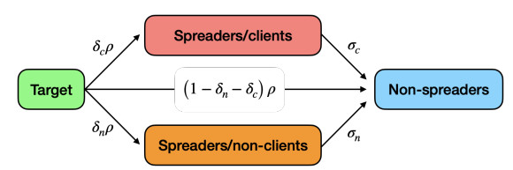
Flow diagram associated to the compartmental model
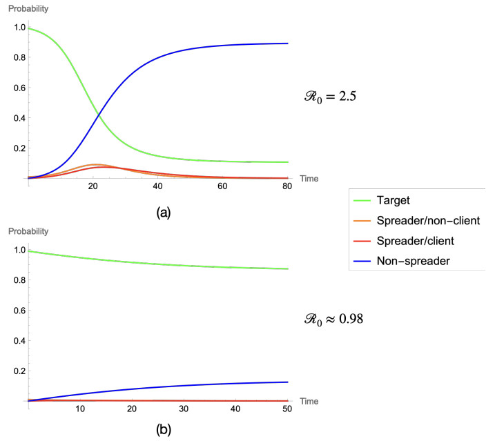
Evolution of the compartment probabilities in two representative simulations of the homogeneous reduced model: (a) Initially supercritical regime, $ \mathcal{R}_{\mathrm{eff}, red}(0) > 1 $; (b) Initially subcritical regime, $ \mathcal{R}_{\mathrm{eff, red}}(0) < 1 $. The parameter values and initial conditions used in each simulation are indicated in the text
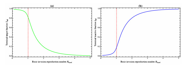
Final campaign size as a function of the basic invasion reproduction number $ \mathcal R_{0, red} $ for the homogeneous reduced model: (a) Terminal target fraction $ T_\infty $; (b) Terminal inactive fraction $ I_\infty = 1-T_\infty $. The parameters are $ \delta_c = 1 $, $ \delta_n = 0 $, and $ \sigma_c = 1 $, with initial conditions $ T(0) = 0.99 $, $ S_c(0) = 0.01 $, and $ S_n(0) = I(0) = 0 $. The parameter $ \rho $ is varied so that $ \mathcal R_{0, red} = \rho $. The vertical red dashed line indicates the initial invasion threshold $ \mathcal R_{\mathrm{eff}, red}(0) = 1 $, corresponding to $ \mathcal R_{0, red} = 1/T(0) $. The figure illustrates that the invasion threshold and the final campaign size are distinct concepts; $ \mathcal R_{0, red} > 1 $ does not imply $ T_\infty = 0 $
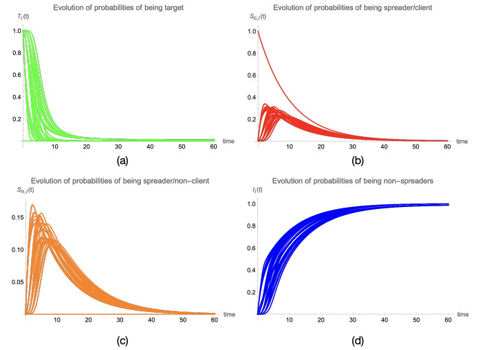
Temporal evolution of the different probabilities in a scale-free complex network with $ m = 1 $ and $ \rho_i = 0.75, \delta_{c, i} = 0.4, \delta_{n, i} = 0.2, \sigma_{c, i} = 0.1, \sigma_{n, i} = 0.1 $: (a) Evolution of the probabilities to be target. (b) Temporal evolution of the probabilities to be spreader/client. (c) Temporal evolution of the probabilities to be spreader/nonclient. (d) Temporal evolution of the probabilities to be nonspreader (client or nonclient)
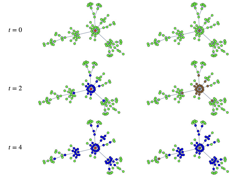
Most-probable-state classification of the network nodes at times $ t = 0, 2, 4 $. Left column: Classification based on the four probabilities $ T_i $, $ S_{c, i} $, $ S_{n, i} $, and $ I_i $. Right column: Classification based on the three aggregated probabilities $ T_i $, $ S_{c, i}+S_{n, i} $, and $ I_i $. The colors indicate the categories defined by each classification rule, not the actual stochastic states of the nodes
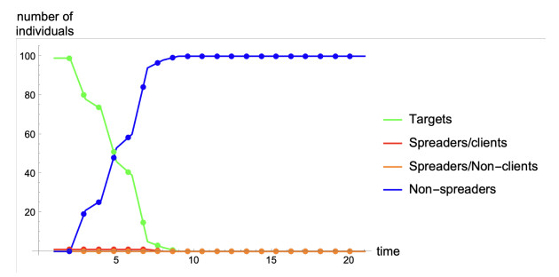
Temporal evolution of the number of nodes classified according to their most probable state. The curves represent classification counts rather than expected compartment sizes
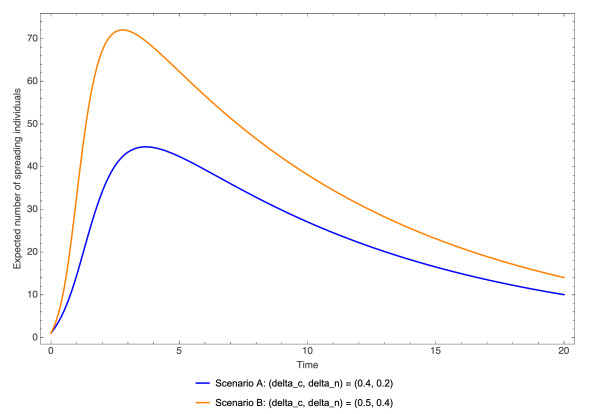
Evolution of the expected number of spreading individuals in two scenarios with different branching probabilities on the same realization of a Barabási–Albert network ($ N = 100 $, $ m = 2 $). Scenario A (blue): $ (\delta_c, \delta_n) = (0.4, 0.2) $. Scenario B (orange): $ (\delta_c, \delta_n) = (0.5, 0.4) $
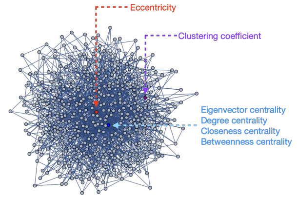
Scale-free network defined by $ m = 3 $ and $ N = 500 $ nodes, where the initial spreader nodes are highlighted in different colors
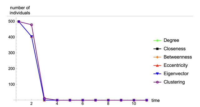
Temporal evolution of the number of nodes classified as targets according to the most-probable-state rule for different choices of the initially spreading node
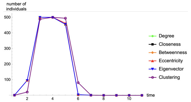
Temporal evolution of the number of nodes classified as spreaders according to the aggregated most-probable-state rule for different choices of the initially spreading node
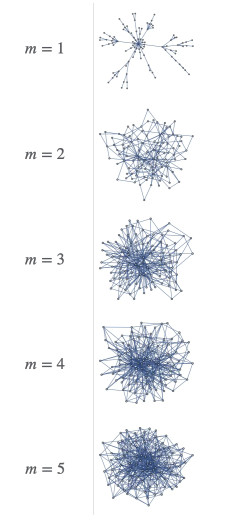
Scale-free networks used in the simulations
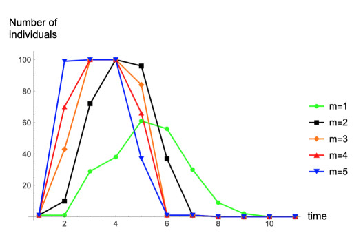
Temporal evolution of the number of nodes classified as spreaders according to the most-probable-state rule for Barabási–Albert networks with different attachment parameters $ m = 1, 2, 3, 4, 5 $. A node is classified as a spreader when its aggregated spreading probability $ S_{c, i}(t)+S_{n, i}(t) $ is greater than both $ T_i(t) $ and $ I_i(t) $. The curves represent classification counts rather than expected compartment sizes




 DownLoad: