The finite volume element method for non-stationary Stokes equations with an LC element pair

Jiehua Zhang; Jiehua Zhang

doi:10.3934/math.2025591

AIMS Mathematics

2025, Volume 10, Issue 6: 13166-13203. doi: 10.3934/math.2025591

Previous Article Next Article

Research article

The finite volume element method for non-stationary Stokes equations with an LC element pair

Jiehua Zhang ^,

School of Science, Kaili University, Guizhou 556011, China

Received: 25 January 2025 Revised: 06 May 2025 Accepted: 09 May 2025 Published: 09 June 2025
MSC : 65N08, 65N12, 65N15, 76D05, 76D07

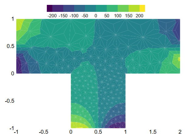
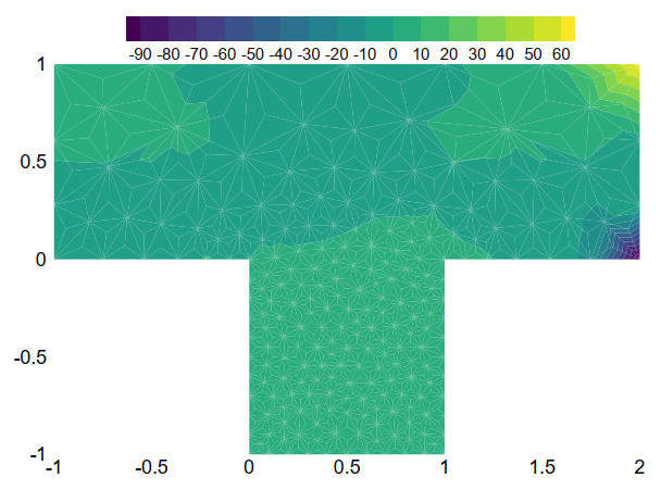
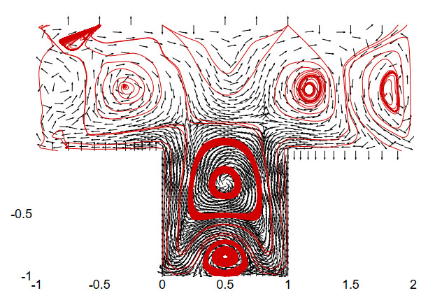
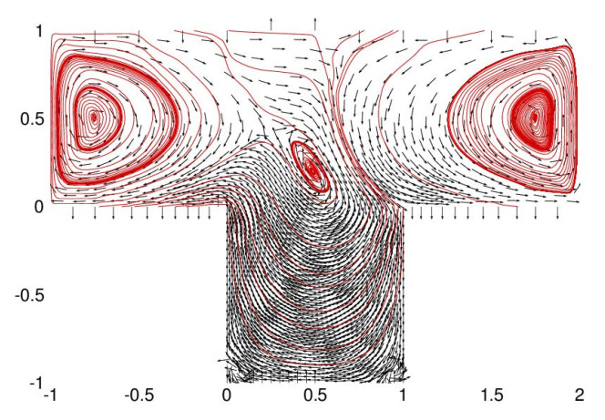
This paper proposes and analyzes a fully discrete spatial-temporal finite volume element method, which employs the LC element pair, for solving non-stationary Stokes equations on barycenter-refined triangular meshes. The proposed scheme utilizes an implicit first-order temporal discretization and is devoid of stabilization parameters. In terms of spatial discretization, the velocity is approximated using a quadratic conforming finite element space, while the pressure is approximated with a discontinuous piecewise linear function space. By utilizing a one-to-many mapping between the trial and test spaces for the velocity components in the finite volume element method, the equivalence between the bilinear forms resulting from the gradient and divergence operators is established, and thus under the mild restrictions of triangular meshes, the stability of the proposed scheme is demonstrated. By introducing a Stokes projection, error estimates for the proposed scheme are obtained. To validate the feasibility and efficiency of the proposed scheme, numerical experiments are presented for the non-stationary Stokes equations.
- finite volume element method,
- local mass conservation,
- non-stationary Stokes equations,
- LC element
Citation: Jiehua Zhang. The finite volume element method for non-stationary Stokes equations with an LC element pair[J]. AIMS Mathematics, 2025, 10(6): 13166-13203. doi: 10.3934/math.2025591

Related Papers:

Abstract

This paper proposes and analyzes a fully discrete spatial-temporal finite volume element method, which employs the LC element pair, for solving non-stationary Stokes equations on barycenter-refined triangular meshes. The proposed scheme utilizes an implicit first-order temporal discretization and is devoid of stabilization parameters. In terms of spatial discretization, the velocity is approximated using a quadratic conforming finite element space, while the pressure is approximated with a discontinuous piecewise linear function space. By utilizing a one-to-many mapping between the trial and test spaces for the velocity components in the finite volume element method, the equivalence between the bilinear forms resulting from the gradient and divergence operators is established, and thus under the mild restrictions of triangular meshes, the stability of the proposed scheme is demonstrated. By introducing a Stokes projection, error estimates for the proposed scheme are obtained. To validate the feasibility and efficiency of the proposed scheme, numerical experiments are presented for the non-stationary Stokes equations.

References

[1]	Z. Chen, J. Wu, Y. Xu, Higher-order finite volume methods for elliptic boundary value problems, Adv. Comput. Math., 37 (2012), 191–253. https://link.springer.com/article/10.1007/s10444-011-9201-8
[2]	Z. Chen, Y. Xu, Y. Zhang, A construction of higher-order finite volume methods, Math. Comp., 84 (2015), 599–628. https://www.ams.org/journals/mcom/2015-84-292/S0025-5718-2014-02881-0/
[3]	S. H. Chou, D. Y. Kwak, Analysis and convergence of a MAC-like scheme for the generalized Stokes problem, Numer. Methods Partial Differential Eq., 13 (1997), 147–162. https://onlinelibrary.wiley.com/doi/abs/10.1002/(SICI)1098-2426(199703)13: 2
[4]	S. H. Chou, P. Vassilevski, A general mixed covolume framework for constructing conservative schemes for elliptic problems, Math. Comp., 68 (1999), 991–1011. https://www.ams.org/journals/mcom/1999-68-227/S0025-5718-99-01090-X/
[5]	R. E. Bank, D. J. Rose, Some error estimates for the box method, SIAM J. Numer. Anal., 24 (1987), 777–787. https://epubs.siam.org/doi/abs/10.1137/0724050
[6]	W. Hackbusch, On first and second order box schemes, Computing, 41 (1989), 277–296. https://link.springer.com/article/10.1007/BF02241218
[7]	R. Li, Z. Chen, W. Wu, Generalized difference methods for differential equations: numerical analysis of finite volume methods, 1 Eds., Boca Raton: CRC Press, 2000. https://doi.org/10.1201/9781482270211
[8]	L. S. K. Fung, A. D. Hiebert, L. X. Nghiem, Reservoir simulation with a control-volume finite-element method, SPE Reserv. Eval. Eng., 7 (1992), 349. https://doi.org/10.2118/21224-PA doi: 10.2118/21224-PA
[9]	Z. Chen, On the control volume finite element methods and their applications to multiphase flow, Netw. Heterog. Media, 1 (2006), 689–706. https://www.aimsciences.org/article/doi/10.3934/nhm.2006.1.689
[10]	M. Schneider, T. Koch, Stable and locally mass-and momentum-conservative control-volume finite-element schemes for the Stokes problem, Comput. Methods Appl. Mech. Eng., 420 (2024), 116723. http://dx.doi.org/10.1016/j.cma.2024.116723 doi: 10.1016/j.cma.2024.116723
[11]	J. Li, Z. Chen, A new stabilized finite volume method for the stationary Stokes equations, Adv. Comput. Math., 30 (2009), 141–152. https://link.springer.com/article/10.1007/s10444-007-9060-5
[12]	M. Yang, H. Song, A postprocessing finite volume element method for time-dependent Stokes equations, Appl. Numer. Math., 59 (2009), 1922–1932. https://doi.org/10.1016/j.apnum.2009.02.004 doi: 10.1016/j.apnum.2009.02.004
[13]	G. He, Y. Zhang, The optimal error estimate of the fully discrete locally stabilized finite volume method for the non-stationary Navier-Stokes problem, Entropy, 24 (2022), 768. http://dx.doi.org/10.3390/e24060768 doi: 10.3390/e24060768
[14]	Z. Luo, A new finite volume element formulation for the non-stationary Navier-Stokes equations, Adv. Appl. Math. Mech., 6 (2014), 615–636. https://doi.org/10.4208/aamm.2013.m83 doi: 10.4208/aamm.2013.m83
[15]	L. Shen, J. Li, Z. Chen, Analysis of a stabilized finite volume method for the transient stokes equations, Int. J. Numer. Anal. Model., 6 (2009), 505–519.
[16]	J. Li, Z. Chen, On the semi-discrete stabilized finite volume method for the transient Navier-Stokes equations, Adv. Comput. Math., 38 (2013), 281–320. https://link.springer.com/article/10.1007/s10444-011-9237-9
[17]	D. Boffi, Stability of higher order triangular Hood-Taylor methods for the stationary Stokes equations, Math. Mod. Meth. Appl. S., 4 (1994), 223–235. https://www.worldscientific.com/doi/abs/10.1142/S0218202594000133
[18]	F. Brezzi, R. S. Falk, Stability of higher-order Hood-Taylor methods, SIAM J. Numer. Anal., 28 (1991), 581–590. https://epubs.siam.org/doi/abs/10.1137/0728032
[19]	D. F. Griffiths, The effect of pressure approximations on finite element calculations of incompressible flows, Department of Mathematical Sciences, University of Dundee, 1982.
[20]	R. W. Thatcher, Locally mass-conserving Taylor-Hood elements for two-and three-dimensional flow, Int. J. Numer. Methods Fluids, 11 (1990), 341–353. https://doi.org/10.1002/fld.1650110307 doi: 10.1002/fld.1650110307
[21]	M. Fabien, J. Guzm$\acute{a}$n, M. Neilan, et al., Low-order divergence-free approximations for the Stokes problem on Worsey-Farin and Powell-Sabin splits, Comput. Meth. Appl. Mech. Eng., 390 (2022), 114444. http://dx.doi.org/10.1016/j.cma.2022.114444 doi: 10.1016/j.cma.2022.114444
[22]	R. W. Thatcher, D. J. Silvester, A locally mass conserving quadratic velocity, linear pressure element, arXiv preprint arXiv: 2001.11878, 2020. https://doi.org/10.48550/arXiv.2001.11878
[23]	D. Boffi, N. Cavallini, F. Gardini, et al., Local mass conservation of Stokes finite elements, J. Sci. Comput., 52 (2012), 383–400. https://link.springer.com/article/10.1007/s10915-011-9549-4
[24]	V. John, A. Linke, C. Merdon, M. Neilan, L. G. Rebholz, On the divergence constraint in mixed finite element methods for incompressible flows, SIAM Rev., 59 (2017), 492–544. https://doi.org/10.1137/15M1047696 doi: 10.1137/15M1047696
[25]	J. Zhang, A family of quadratic finite volume method for solving the Stokes equation, Comput. Math. Appl., 117 (2022), 155–186. https://doi.org/10.1016/j.camwa.2022.04.014 doi: 10.1016/j.camwa.2022.04.014
[26]	D. N. Arnold, J. Qin, Quadratic velocity / linear pressure Stokes elements, Adv. Comput. Meth. Partial Differ. Eq., 7 (1992), 28–34.
[27]	J. Guzm$\acute{a}$n, M. Neilan, Inf-sup stable finite elements on barycentric refinements producing divergence–free approximations in arbitrary dimensions, SIAM J. Numer. Anal., 56 (2018), 2826–2844. https://doi.org/10.1137/17M1153467 doi: 10.1137/17M1153467
[28]	Y. Lou, H. Rui, A quadratic discontinuous finite volume element scheme for stokes problems, J. Sci. Comput., 99 (2024), 44. https://link.springer.com/article/10.1007/s10915-024-02506-4
[29]	H. Yang, Y. Li, The mixed finite volume methods for Stokes problem based on MINI element pair, Int. J. Numer. Anal. Model., 20 (2022), 134.
[30]	Y. Zhou, J. Wu, A family of quadratic finite volume element schemes over triangular meshes for elliptic equations, Comput. Math. Appl., 79 (2020), 2473–2491. https://doi.org/10.1016/j.camwa.2019.11.01 doi: 10.1016/j.camwa.2019.11.01
[31]	Y. Zhou, J. Wu, A unified analysis of a class of quadratic finite volume element schemes on triangular meshes, Adv. Comput. Math., 46 (2020), 1–31. https://link.springer.com/article/10.1007/s10444-020-09809-8
[32]	Y. Zhou, J. Wu, A family of quadratic finite volume element schemes for anisotropic diffusion problems on triangular meshes, J. Comput. Appl. Math., 402 (2022), 113794. https://doi.org/10.1016/j.cam.2021.113794 doi: 10.1016/j.cam.2021.113794
[33]	J. G. Heywood, R. Rannacher, Finite element approximation of the nonstationary Navier-Stokes problem. Ⅰ. Regularity of solutions and second-order error estimates for spatial discretization, SIAM J. Numer. Anal., 19 (1982), 275–311. https://doi.org/10.1137/0719018 doi: 10.1137/0719018
[34]	J. G. Heywood, R. Rannacher, Finite-element approximation of the nonstationary Navier-Stokes problem. Part Ⅳ: error analysis for second-order time discretization, SIAM J. Numer. Anal., 27 (1990), 353–384. https://doi.org/10.1137/0727022 doi: 10.1137/0727022
[35]	V. Girault, P. A. Raviart, Finite element methods for Navier-Stokes equations: theory and algorithms, 1 Eds., New York: Springer Science & Business Media, 2012.
[36]	R. W. Clough, Finite element stiffness matricess for analysis of plate bending, Proc. of the First Conf. on Matrix Methods in Struct. Mech. 1965: 515–546.
[37]	M. A. Case, V. J. Ervin, A. Linke, L. G. Rebholz, A connection between Scott-Vogelius and grad-div stabilized Taylor-Hood FE approximations of the Navier-Stokes equations, SIAM J. Numer. Anal., 49 (2011), 1461–1481. https://doi.org/10.1137/100794250 doi: 10.1137/100794250
[38]	M. Neilan, A. Zytoon, Connection between grad-div stabilized Stokes finite elements and divergence-free Stokes finite elements, Int. J. Numer. Anal. Model., 17 (2020).
[39]	F. Brezzi, On the existence, uniqueness and approximation of saddlepoint problems arising from Lagrangian multipliers, Publ. S$\acute{e}$min. Math. Inform. Rennes, S4 (1974), 1–26.
[40]	R. A. Nicolaides, Existence, uniqueness and approximation for generalized saddle point problems, SIAM J. Numer. Anal., 19 (1982), 349–357. https://doi.org/10.1137/0719021 doi: 10.1137/0719021
[41]	J. Zhang, Z. Chen, $\mathrm{L}^2$ error estimates for a family of cubic finite volume methods on triangular meshes, Comput. Math. Appl., 143 (2023), 189–223. https://doi.org/10.1016/j.camwa.2023.04.038 doi: 10.1016/j.camwa.2023.04.038
[42]	Q. Zou, An unconditionally stable quadratic finite volume scheme over triangular meshes for elliptic equations, J. Sci. Comput., 70 (2017), 112–124. https://link.springer.com/article/10.1007/s10915-016-0244-3
[43]	Y. He, K. Li, Convergence and stability of finite element nonlinear Galerkin method for the Navier-Stokes equations, Numer. Math., 79 (1998), 77–106. https://link.springer.com/article/10.1007/s002110050332
[44]	J. Shen, Long time stability and convergence for fully discrete nonlinear Galerkin methods, Appl. Anal., 38 (1990), 201–229. https://doi.org/10.1080/00036819008839963 doi: 10.1080/00036819008839963
[45]	P. N. Shankar, M. D. Deshpande, Fluid mechanics in the driven cavity, Annu. Rev. Fluid Mech., 32 (2000), 93–136. https://doi.org/10.1146/annurev.fluid.32.1.93 doi: 10.1146/annurev.fluid.32.1.93

Reader Comments

Your name:*

Email:*
© 2025 the Author(s), licensee AIMS Press. This is an open access article distributed under the terms of the Creative Commons Attribution License (http://creativecommons.org/licenses/by/4.0)