Significant results in the $ \mathrm{p} $th moment for Hilfer fractional stochastic delay differential equations

Wedad Albalawi; Muhammad Imran Liaqat; Fahim Ud Din; Kottakkaran Sooppy Nisar; Abdel-Haleem Abdel-Aty; Wedad Albalawi; Muhammad Imran Liaqat; Fahim Ud Din; Kottakkaran Sooppy Nisar; Abdel-Haleem Abdel-Aty

doi:10.3934/math.2025451

AIMS Mathematics

2025, Volume 10, Issue 4: 9852-9881. doi: 10.3934/math.2025451

Previous Article Next Article

Research article Special Issues

Significant results in the $ \mathrm{p} $th moment for Hilfer fractional stochastic delay differential equations

1.
Department of Mathematical Sciences, College of Science, Princess Nourah bint Abdulrahman University, P.O. Box 84428, Riyadh 11671, Saudi Arabia
2.
Abdus Salam School of Mathematical Sciences, Government College University, 68-B, New Muslim Town, Lahore 54600, Pakistan
3.
Department of Decision Sciences, SK-Hub-Oxford Business College, OX1 2EP, Oxford, UK
4.
Department of Mathematics, College of Science and Humanities in Al-Kharj, Prince Sattam Bin Abdulaziz University, Al-Kharj 11942, Saudi Arabia
5.
Department of Physics, College of Sciences, University of Bisha, Bisha 61922, Saudi Arabia

Received: 14 January 2025 Revised: 26 March 2025 Accepted: 15 April 2025 Published: 27 April 2025
MSC : 34A07, 34A08, 60G22

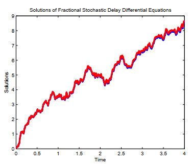
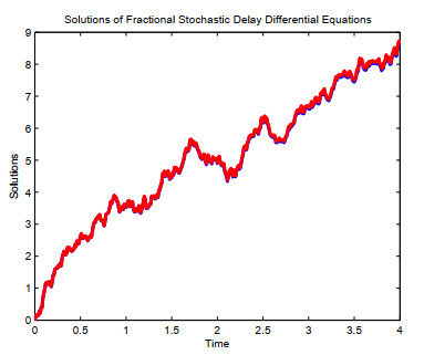
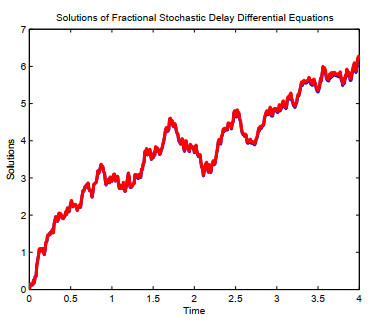
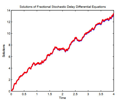
Well-posedness is crucial in studying fractional stochastic differential equations, as it ensures that solutions are mathematically sound and applicable to practical situations. A well-formulated model satisfies the essential requirements for solutions, such as existence, uniqueness, and stability concerning various parameters. Using fixed-point theory, we prove that the solution to stochastic fractional delay differential equations with the Hilfer fractional operator exists, is unique, and continuously depends on the initial values and the fractional derivative. Additionally, we establish a smoothness theorem for the solution and demonstrate that the solution of the original system converges to the averaged system in the $ \mathrm{p} $th moment. Last, to support our theoretical findings, we provide examples and graphical illustrations. The primary tools used in our proofs include the Burkholder-Davis-Gundy inequality, Jensen's inequality, and Hölder's inequality.
- averaging principle,
- Hilfer fractional derivative,
- well-posedness,
- contraction mapping principle,
- regularity
Citation: Wedad Albalawi, Muhammad Imran Liaqat, Fahim Ud Din, Kottakkaran Sooppy Nisar, Abdel-Haleem Abdel-Aty. Significant results in the $ \mathrm{p} $th moment for Hilfer fractional stochastic delay differential equations[J]. AIMS Mathematics, 2025, 10(4): 9852-9881. doi: 10.3934/math.2025451

Related Papers:

Abstract

Well-posedness is crucial in studying fractional stochastic differential equations, as it ensures that solutions are mathematically sound and applicable to practical situations. A well-formulated model satisfies the essential requirements for solutions, such as existence, uniqueness, and stability concerning various parameters. Using fixed-point theory, we prove that the solution to stochastic fractional delay differential equations with the Hilfer fractional operator exists, is unique, and continuously depends on the initial values and the fractional derivative. Additionally, we establish a smoothness theorem for the solution and demonstrate that the solution of the original system converges to the averaged system in the $ \mathrm{p} $th moment. Last, to support our theoretical findings, we provide examples and graphical illustrations. The primary tools used in our proofs include the Burkholder-Davis-Gundy inequality, Jensen's inequality, and Hölder's inequality.

References

[1]	M. M. Raja, V. Vijayakumar, K. C. Veluvolu, A. Shukla, K. S. Nisar, Existence and optimal control results for Caputo fractional delay Clark's subdifferential inclusions of order $r\in(1, 2)$ with sectorial operators, Optim. Control Appl. Methods, 45 (2024), 1832–1850. https://doi.org/10.1002/oca.3125 doi: 10.1002/oca.3125
[2]	M. M. Raja, V. Vijayakumar, K. C. Veluvolu, An analysis on approximate controllability results for impulsive fractional differential equations of order $1 < r < 2$ with infinite delay using sequence method, Math. Methods Appl. Sci., 47 (2024), 336–351. https://doi.org/10.1002/mma.9657 doi: 10.1002/mma.9657
[3]	Y. K. Ma, M. M. Raja, A. Shukla, V. Vijayakumar, K. S. Nisar, K. Thilagavathi, New results on approximate controllability of fractional delay integrodifferential systems of order $1 < r < 2$ with Sobolev-type, Alex. Eng. J., 81 (2023), 501–518. https://doi.org/10.1016/j.aej.2023.09.043 doi: 10.1016/j.aej.2023.09.043
[4]	M. I. Liaqat, S. Etemad, S. Rezapour, C. Park, A novel analytical Aboodh residual power series method for solving linear and nonlinear time-fractional partial differential equations with variable coefficients, AIMS Math., 7 (2022), 16917–16948. https://doi.org/10.3934/math.2022929 doi: 10.3934/math.2022929
[5]	Y. Luchko, Fractional differential equations with the general fractional derivatives of arbitrary order in the Riemann-Liouville sense, Mathematics, 10 (2022), 1–24. https://doi.org/10.3390/math10060849 doi: 10.3390/math10060849
[6]	M. I. Liaqat, A. Akgül, M. Bayram, Series and closed form solution of Caputo time-fractional wave and heat problems with the variable coefficients by a novel approach, Opt. Quantum Electron., 56 (2024), 203. https://doi.org/10.1007/s11082-023-05751-3 doi: 10.1007/s11082-023-05751-3
[7]	R. Hilfer, Applications of fractional calculus in physics, World Scientific, 2000.
[8]	D. Raghavan, J. F. Gómez-Aguilar, N. Sukavanam, Analytical approach of Hilfer fractional order differential equations using iterative Laplace transform method, J. Math. Chem., 61 (2023), 219–241. https://doi.org/10.1007/s10910-022-01419-7 doi: 10.1007/s10910-022-01419-7
[9]	F. Li, C. L. Wang, H. W. Wang, Existence results for Hilfer fractional differential equations with variable coefficient, Fractal Fract., 6 (2022), 1–15. https://doi.org/10.3390/fractalfract6010011 doi: 10.3390/fractalfract6010011
[10]	S. G. Zhu, H. W. Wang, F. Li, Solutions for Hilfer-type linear fractional integro-differential equations with a variable coefficient, Fractal Fract., 8 (2024), 1–15. https://doi.org/10.3390/fractalfract8010063 doi: 10.3390/fractalfract8010063
[11]	P. Bedi, A. Kumar, T. Abdeljawad, A. Khan, Existence of mild solutions for impulsive neutral Hilfer fractional evolution equations, Adv. Differ. Equ., 2020 (2020), 1–16. https://doi.org/10.1186/s13662-020-02615-y doi: 10.1186/s13662-020-02615-y
[12]	R. Kasinathan, R. Kasinathan, D. Baleanu, A. Annamalai, Hilfer fractional neutral stochastic differential equations with non-instantaneous impulses, AIMS Math., 6 (2021), 4474–4491. https://doi.org/10.3934/math.2021265 doi: 10.3934/math.2021265
[13]	J. Y. Lv, X. Y. Yang, A class of Hilfer fractional stochastic differential equations and optimal controls, Adv. Differ. Equ., 2019 (2019), 17. https://doi.org/10.1186/s13662-019-1953-3 doi: 10.1186/s13662-019-1953-3
[14]	Y. H. Jin, W. C. He, L. Y. Wang, J. Mu, Existence of mild solutions to delay diffusion equations with Hilfer fractional derivative, Fractal Fract., 8 (2024), 1–15. https://doi.org/10.3390/fractalfract7100724 doi: 10.3390/fractalfract7100724
[15]	K. Karthikeyan, P. R. Sekar, P. Karthikeyan, A. Kumar, T. Botmart, W. Weera, A study on controllability for Hilfer fractional differential equations with impulsive delay conditions, AIMS Math., 8 (2023), 4202–4219. https://doi.org/10.3934/math.2023209 doi: 10.3934/math.2023209
[16]	A. Hegade, S. Bhalekar, Stability analysis of Hilfer fractional-order differential equations, Eur. Phys. J. Spec. Top., 232 (2023), 2357–2365. https://doi.org/10.1140/epjs/s11734-023-00960-z doi: 10.1140/epjs/s11734-023-00960-z
[17]	T. K. Yuldashev, B. J. Kadirkulovich, Nonlocal problem for a mixed type fourth-order differential equation with Hilfer fractional operator, Ural Math. J., 6 (2020), 153–167. http://dx.doi.org/10.15826/umj.2020.1.013 doi: 10.15826/umj.2020.1.013
[18]	M. R. Admon, N. Senu, A. Ahmadian, Z. A. Majid, S. Salahshour, A new accurate method for solving fractional relaxation-oscillation with Hilfer derivatives, Comput. Appl. Math., 42 (2023), 10. https://doi.org/10.1007/s40314-022-02154-0 doi: 10.1007/s40314-022-02154-0
[19]	I. M. Batiha, A. A. Abubaker, I. H. Jebril, S. B. Al-Shaikh, K. Matarneh, A numerical approach of handling fractional stochastic differential equations, Axioms, 12 (2023), 1–12. https://doi.org/10.3390/axioms12040388 doi: 10.3390/axioms12040388
[20]	J. H. Chen, S. Ke, X. F. Li, W. B. Liu, Existence, uniqueness and stability of solutions to fractional backward stochastic differential equations, Appl. Math. Sci. Eng., 30 (2022), 811–829. https://doi.org/10.1080/27690911.2022.2142219 doi: 10.1080/27690911.2022.2142219
[21]	S. Moualkia, Y. Xu, On the existence and uniqueness of solutions for multidimensional fractional stochastic differential equations with variable order, Mathematics, 9 (2021), 1–12. https://doi.org/10.3390/math9172106 doi: 10.3390/math9172106
[22]	A. Ali, K. Hayat, A. Zahir, K. Shah, T. Abdeljawad, Qualitative analysis of fractional stochastic differential equations with variable order fractional derivative, Qual. Theory Dyn. Syst., 23 (2024), 120. https://doi.org/10.1007/s12346-024-00982-5 doi: 10.1007/s12346-024-00982-5
[23]	S. Li, S. U. Khan, M. B. Riaz, S. A. AlQahtani, A. M. Alamri, Numerical simulation of a fractional stochastic delay differential equations using spectral scheme: a comprehensive stability analysis, Sci. Rep., 14 (2024), 6930. https://doi.org/10.1038/s41598-024-56944-z doi: 10.1038/s41598-024-56944-z
[24]	W. Albalawi, M. I. Liaqat, F. U. Din, K. S. Nisar, A. H. Abdel-Aty, Well-posedness and Ulam-Hyers stability results of solutions to pantograph fractional stochastic differential equations in the sense of conformable derivatives, AIMS Math., 9 (2024), 12375–12398. https://doi.org/10.3934/math.2024605 doi: 10.3934/math.2024605
[25]	T. S. Doan, P. T. Huong, P. E. Kloeden, A. M. Vu, Euler-Maruyama scheme for Caputo stochastic fractional differential equations, J. Comput. Appl. Math., 380 (2020), 112989. https://doi.org/10.1016/j.cam.2020.112989 doi: 10.1016/j.cam.2020.112989
[26]	P. Umamaheswari, K. Balachandran, N. Annapoorani, Existence and stability results for Caputo fractional stochastic differential equations with Lévy noise, Filomat, 34 (2020), 1739–1751. https://doi.org/10.2298/FIL2005739U doi: 10.2298/FIL2005739U
[27]	M. Li, Y. J. Niu, J. Zou, A result regarding finite-time stability for Hilfer fractional stochastic differential equations with delay, Fractal Fract., 7 (2023), 1–16. https://doi.org/10.3390/fractalfract7080622 doi: 10.3390/fractalfract7080622
[28]	M. Abouagwa, R. A. R. Bantan, W. Almutiry, A. D. Khalaf, M. Elgarhy, Mixed Caputo fractional neutral stochastic differential equations with impulses and variable delay, Fractal Fract., 5 (2021), 1–19. https://doi.org/10.3390/fractalfract5040239 doi: 10.3390/fractalfract5040239
[29]	W. Albalawi, M. I. Liaqat, F. U. Din, K. S. Nisar, A. H. Abdel-Aty, The analysis of fractional neutral stochastic differential equations in space, AIMS Math., 9 (2024), 17386–17413. https://doi.org/10.3934/math.2024845 doi: 10.3934/math.2024845
[30]	M. I. Liaqat, F. U. Din, W. Albalawi, K. S. Nisar, A. H. Abdel-Aty, Analysis of stochastic delay differential equations in the framework of conformable fractional derivatives, AIMS Math., 9 (2024), 11194–11211. https://doi.org/10.3934/math.2024549 doi: 10.3934/math.2024549
[31]	Z. A. Khan, M. I. Liaqat, A. Akgül, J. A. Conejero, Qualitative analysis of stochastic Caputo-Katugampola fractional differential equations, Axioms, 13 (2024), 1–27. https://doi.org/10.3390/axioms13110808 doi: 10.3390/axioms13110808
[32]	R. Kasinathan, R. Kasinathan, D. Baleanu, A. Annamalai, Well posedness of second-order impulsive fractional neutral stochastic differential equations, AIMS Math., 6 (2021), 9222–9235. https://doi.org/10.3934/math.2021536 doi: 10.3934/math.2021536
[33]	J. Zou, D. F. Luo, M. M. Li, The existence and averaging principle for stochastic fractional differential equations with impulses, Math. Methods Appl. Sci., 46 (2023), 6857–6874. https://doi.org/10.1002/mma.8945 doi: 10.1002/mma.8945
[34]	J. Zou, D. F. Luo, A new result on averaging principle for Caputo-type fractional delay stochastic differential equations with Brownian motion, Appl. Anal., 103 (2024), 1397–1417. https://doi.org/10.1080/00036811.2023.2245845 doi: 10.1080/00036811.2023.2245845
[35]	J. Zou, D. F. Luo, On the averaging principle of Caputo type neutral fractional stochastic differential equations, Qual. Theory Dyn. Syst., 23 (2024), 82. https://doi.org/10.1007/s12346-023-00916-7 doi: 10.1007/s12346-023-00916-7
[36]	W. Mao, S. R. You, X. Q. Wu, X. R. Mao, On the averaging principle for stochastic delay differential equations with jumps, Adv. Differ. Equ., 2015 (2015), 1–19.
[37]	W. J. Xu, W. Xu, K. Lu, An averaging principle for stochastic differential equations of fractional order $0< \alpha<1$, Fract. Calc. Appl. Anal., 23 (2020), 908–919. https://doi.org/10.1515/fca-2020-0046 doi: 10.1515/fca-2020-0046
[38]	Z. K. Guo, G. Y. Lv, J. L. Wei, Averaging principle for stochastic differential equations under a weak condition, Chaos, 30 (2020), 123139. https://doi.org/10.1063/5.0031030 doi: 10.1063/5.0031030
[39]	J. K. Liu, W. Xu, An averaging result for impulsive fractional neutral stochastic differential equations, Appl. Math. Lett., 114 (2021), 106892. https://doi.org/10.1016/j.aml.2020.106892 doi: 10.1016/j.aml.2020.106892
[40]	J. K. Liu, W. Xu, Q. Guo, Averaging principle for impulsive stochastic partial differential equations, Stoch. Dyn., 21 (2021), 2150014. https://doi.org/10.1142/S0219493721500143 doi: 10.1142/S0219493721500143
[41]	H. M. Ahmed, Q. X. Zhu, The averaging principle of Hilfer fractional stochastic delay differential equations with Poisson jumps, Appl. Math. Lett., 112 (2021), 106755. https://doi.org/10.1016/j.aml.2020.106755 doi: 10.1016/j.aml.2020.106755
[42]	W. J. Xu, W. Xu, S. Zhang, The averaging principle for stochastic differential equations with Caputo fractional derivative, Appl. Math. Lett., 93 (2019), 79–84. https://doi.org/10.1016/j.aml.2019.02.005 doi: 10.1016/j.aml.2019.02.005
[43]	Y. Y. Jing, Z. Li, Averaging principle for backward stochastic differential equations, Discrete Dyn. Nat. Soc., 2021 (2021), 6615989. https://doi.org/10.1155/2021/6615989 doi: 10.1155/2021/6615989
[44]	A. M. Djaouti, Z. A. Khan, M. I. Liaqat, A. Al-Quran, Existence, uniqueness, and averaging principle of fractional neutral stochastic differential equations in the $L^{p}$ space with the framework of the $\Psi$-Caputo derivative, Mathematics, 12 (2024), 1–20. https://doi.org/10.3390/math12071037 doi: 10.3390/math12071037
[45]	M. Mouy, H. Boulares, S. Alshammari, M. Alshammari, Y. Laskri, W. W. Mohammed, On averaging principle for Caputo-Hadamard fractional stochastic differential pantograph equation, Fractal Fract., 7 (2023), 1–9. https://doi.org/10.3390/fractalfract7010031 doi: 10.3390/fractalfract7010031
[46]	J. K. Liu, W. Wei, J. B. Wang, W. Xu, Limit behavior of the solution of Caputo-Hadamard fractional stochastic differential equations, Appl. Math. Lett., 140 (2023), 108586. https://doi.org/10.1016/j.aml.2023.108586 doi: 10.1016/j.aml.2023.108586
[47]	J. K. Liu, H. D. Zhang, J. B. Wang, C. Jin, J. Li, W. Xu, A note on averaging principles for fractional stochastic differential equations, Fractal Fract., 8 (2024), 1–9. https://doi.org/10.3390/fractalfract8040216 doi: 10.3390/fractalfract8040216
[48]	D. D. Yang, J. F. Wang, C. Z. Bai, Averaging principle for $\psi$-Capuo fractional stochastic delay differential equations with Poisson jumps, Symmetry, 15 (2023), 1–15. https://doi.org/10.3390/sym15071346 doi: 10.3390/sym15071346
[49]	A. A. Kilbas, H. M. Srivastava, J. J. Trujillo, Theory and applications of fractional differential equations, Elsevier, 2006.
[50]	M. I. Liaqat, F. U. Din, A. Akgül, M. B. Riaz, Some important results for the conformable fractional stochastic pantograph differential equations in the $\mathbf{L}^{\mathrm{p}}$ space, J. Math. Comput. Sci., 37 (2025), 106–131. https://doi.org/10.22436/jmcs.037.01.08 doi: 10.22436/jmcs.037.01.08

Reader Comments

Your name:*

Email:*
© 2025 the Author(s), licensee AIMS Press. This is an open access article distributed under the terms of the Creative Commons Attribution License (http://creativecommons.org/licenses/by/4.0)