A new approach to solving local fractional Riccati differential equations using the Adomian-Elzaki method

Hilal Aydemir; Mehmet Merdan; Ümit Demir; Hilal Aydemir; Mehmet Merdan; Ümit Demir

doi:10.3934/math.2025420

AIMS Mathematics

2025, Volume 10, Issue 4: 9122-9149. doi: 10.3934/math.2025420

Previous Article Next Article

Research article Special Issues

A new approach to solving local fractional Riccati differential equations using the Adomian-Elzaki method

1.
Department of Mathematical Engineering, Gumushane University, Gumushane, Turkey
2.
Banking and Insurance Department/Finance, Bayburt University, Bayburt, Turkey

Received: 23 January 2025 Revised: 06 March 2025 Accepted: 20 March 2025 Published: 21 April 2025
MSC : 35C05, 35R11, 65R10

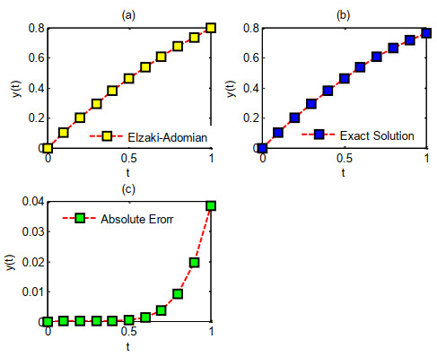
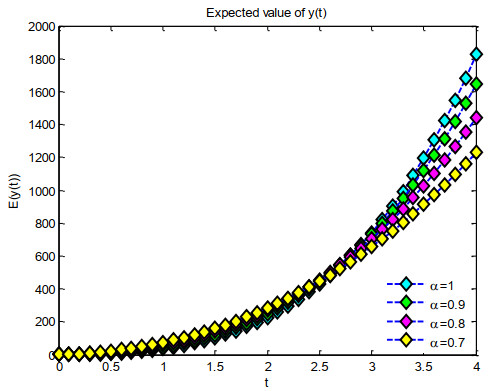
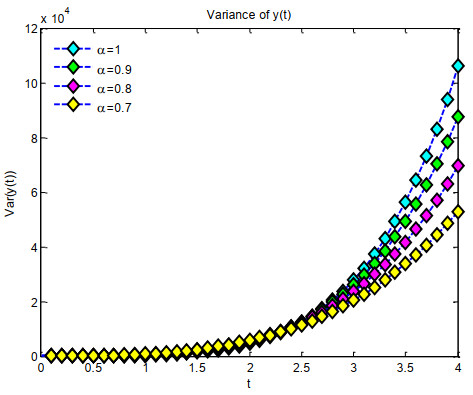
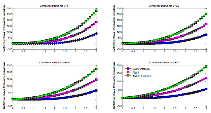
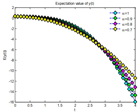
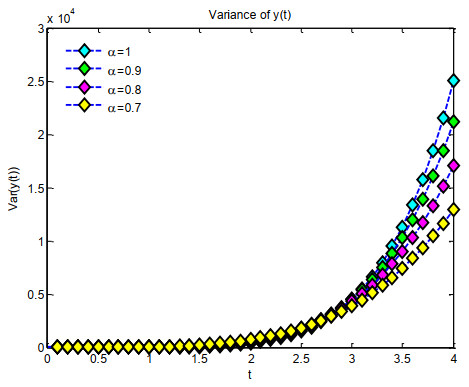
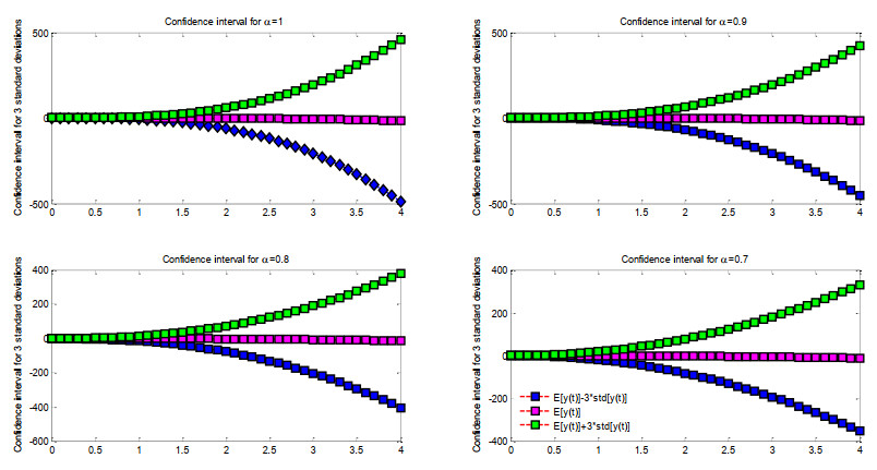
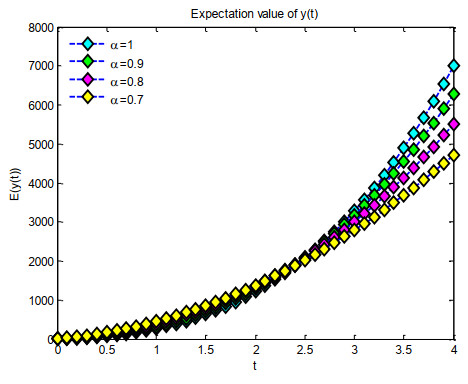
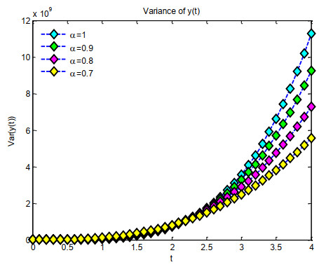
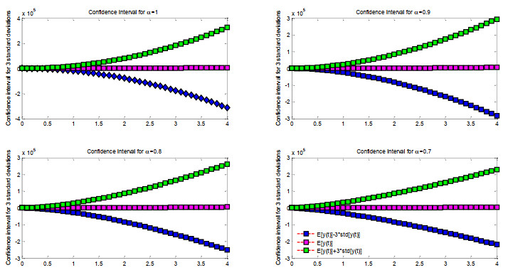
The Elzaki-Adomian decomposition method (EADM) is intended to serve as an efficient analytical method for the resolution of these original fractional-order Riccati differential equations. This can be accomplished permanently by incorporating the Adomian decomposition method with Elzaki. The local fractional derivative is implemented in this format. Particularly in the context of nonlinear differential equations (ODE), this approach is preferred over digital gaps. Additionally, the method's convergence. Random individuals with uniform, beta, normal, and gamma distributions are used to select the initial conditions or coefficients of the equations. The variance, confidence interval, and expected value of the solutions that are obtained will be determined. MATLAB (2013a) package software will be employed to display the individuals that were brought together, and the results will be analyzed randomly.
- local fractional derivative,
- Elzaki-Adomian decomposition method,
- continuous probability distributions,
- expectation value,
- variance
Citation: Hilal Aydemir, Mehmet Merdan, Ümit Demir. A new approach to solving local fractional Riccati differential equations using the Adomian-Elzaki method[J]. AIMS Mathematics, 2025, 10(4): 9122-9149. doi: 10.3934/math.2025420

Related Papers:

Abstract

The Elzaki-Adomian decomposition method (EADM) is intended to serve as an efficient analytical method for the resolution of these original fractional-order Riccati differential equations. This can be accomplished permanently by incorporating the Adomian decomposition method with Elzaki. The local fractional derivative is implemented in this format. Particularly in the context of nonlinear differential equations (ODE), this approach is preferred over digital gaps. Additionally, the method's convergence. Random individuals with uniform, beta, normal, and gamma distributions are used to select the initial conditions or coefficients of the equations. The variance, confidence interval, and expected value of the solutions that are obtained will be determined. MATLAB (2013a) package software will be employed to display the individuals that were brought together, and the results will be analyzed randomly.

References

[1]	S. Momani, N. Shawagfeh, Decomposition method for solving fractional Riccati differential equations, Appl. Math. Comput., 182 (2006), 1083–1092.https://doi.org/10.1016/j.amc.2006.05.008 doi: 10.1016/j.amc.2006.05.008
[2]	M. Merdan, On the solutions fractional Riccati differential equation with modified Riemann-Liouville derivative, Int. J. Differ. Equ., 2012 (2012), 346089.https://doi.org/10.1155/2012/346089 doi: 10.1155/2012/346089
[3]	S. Abbasbandy, Iterated He's homotopy perturbation method for quadratic Riccati differential equation, Appl. Math. Comput., 175 (2006), 581–589.https://doi.org/10.1016/j.amc.2005.07.035 doi: 10.1016/j.amc.2005.07.035
[4]	J. H. He, Approximate analytical solution for seepage flow with fractional derivatives in porous media, Comput. Methods Appl. Mech. Eng., 167 (1998), 57–68.https://doi.org/10.1016/S0045-7825(98)00108-X doi: 10.1016/S0045-7825(98)00108-X
[5]	H. Jafari, H. Tajadodi, He's variational iteration method for solving fractional Riccati differential equation, Int. J. Differ. Equ., 2010 (2010), 764738.https://doi.org/10.1155/2010/764738 doi: 10.1155/2010/764738
[6]	M. M. Khader, Numerical treatment for solving fractional Riccati differential equation, J. Egyptian Math. Soc., 21 (2013), 32–37.https://doi.org/10.1016/j.joems.2012.09.005 doi: 10.1016/j.joems.2012.09.005
[7]	M. M. Khader, A. M. S. Mahdy, E. S. Mohamed, On approximate solutions for fractional Riccati differential equation, Int. J. Eng. Appl. Sci., 4 (2014), 1–10.
[8]	M. M. Khader, On the numerical solutions for the fractional difusion equation, Commun. Nonlinear Sci. Numer. Simul., 16 (2011), 2535–2542.https://doi.org/10.1016/j.cnsns.2010.09.007 doi: 10.1016/j.cnsns.2010.09.007
[9]	T. Khaniyev, M. Merdan, On the fractional Riccati differential equation, Int. J. Pure Appl. Math., 107 (2016), 145–160.https://doi.org//10.12732/ijpam.v107i1.12 doi: 10.12732/ijpam.v107i1.12
[10]	G. Adomian, Solving frontier problems of physics: the decomposition method, Dordrecht: Springer, 1994.https://doi.org/10.1007/978-94-015-8289-6
[11]	G. Adomian, A review of the decomposition method and some recent results for nonlinear equation, Math. Comput. Model., 13 (1990), 17–43.https://doi.org/10.1016/0895-7177(90)90125-7 doi: 10.1016/0895-7177(90)90125-7
[12]	G. Adomian, R. Rach, Noise terms in decomposition solution series, Comput. Math. Appl., 24 (1992), 61–64.
[13]	J. Biazar, S. M. Shafiof, A simple algorithm for calculating Adomian polynomials, Int. J. Contemp. Math. Sciences, 2 (2007), 975–982.
[14]	T. M. Elzaki, S. M. Ezaki, Solution of integro-differential equations by using Elzaki transform, Global J. Math. Sci. Theory Pract., 3 (2011), 1–11.
[15]	T. M. Elzaki, S. M. Ezaki, On the Elzaki transform and higher order ordinary differential equations, Adv. Theor. Appl. Math., 6 (2011), 107–113.
[16]	T. M. Elzaki, S. M. Ezaki, On the Elzaki transform and ordinary differential equation with variable coefficients, Adv. Theor. Appl. Math., 6 (2011), 41–46.
[17]	M. M. A. Mahgob, T. M. Elzaki, Elzaki transform and integro-differential equation with a Bulge function, IOSR J. Math., 11 (2015), 25–28.
[18]	M. M. A. Mahgob, T. M. Elzaki, Solution of partial integro-differential equations by Elzaki transform method, Appl. Math. Sci., 9 (2015), 295–303.https://doi.org/10.12988/ams.2015.411984 doi: 10.12988/ams.2015.411984
[19]	M. M. A. Mahgob, Elzaki transform and a Bulge function on volterra integral equations of the second kind, IOSR J. Math., 11 (2012), 68–70.
[20]	P. K. G. Bhadane, V. H. Pradhan, S. V. Desale, Elzaki transform solution of one dimensional groundwater recharge through spreading, Int. J. Eng. Res. Appl., 3 (2013), 1607–1610.
[21]	T. M. Elzaki, E. M. A. Hilal, Analytical solution for telegraph equation by modified of Sumudu transform "Elzaki transform", Math. Theory Model., 2 (2012), 104–111.
[22]	T. M. Elzaki, S. M. Ezaki, On the Elzaki transform and system of partial differential equations, Adv. Theor. Appl. Math., 6 (2011), 115–123.
[23]	D. Ziane, M. H. Cherif, Resolution of nonlinear partial differential equations by Elzaki transform decomposition method, J. Appro. Theo. Appl. Math., 5 (2015), 17–30.
[24]	N. A. Shah, I. Dassios, J. D. Chung, A decomposition method for a fractional-order multi-dimensional telegraph equation via the Elzaki transform, Symmetry, 13 (2021), 1–12.https://doi.org/10.3390/sym13010008 doi: 10.3390/sym13010008
[25]	E. I. Akinola, F. O. Akinpelu, A. O. Areo, J. O. Oladejo, Ekzaki decompostion method for solving epidemic model, Int. J. Chem. Math. Phys., 1 (2017), 68–72.
[26]	O. E. Ige, R. A. Oderinu, T. M. Elzaki, Adomian polynomial and Elzaki transform method of solving fifth order Korteweg-De Vries equation, Caspian J. Math. Sci., 8 (2019), 103–119.https://doi.org/10.22080/cjms.2018.14486.1346 doi: 10.22080/cjms.2018.14486.1346
[27]	O. E. Ige, R. A. Oderinu, T. M. Elzaki, Adomian polynomial and Elzaki transform method for solving sine-Gordan equations, IAENG Int. J. Appl. Math., 49 (2019), 1–7.
[28]	R. I. Nurudden, Elzaki decomposition method and its applications in solving linear and nonlinear Schrödinger equations, Sohag J. Math., 4 (2017), 1–5.https://doi.org/10.18576/sjm/040201 doi: 10.18576/sjm/040201
[29]	A. C. Versoliwala, T. R. Singh, An approximate analytical solution of non linear partial differential equation for water infiltration in unsaturated soils by combined Elzaki transform and Adomian decomposition method, J. Phys. Conf. Ser., 1473 (2020), 012009.https://doi.org/10.1088/1742-6596/1473/1/012009 doi: 10.1088/1742-6596/1473/1/012009
[30]	M. Sadaf, Z. Perveen, G. Akram, U. Habiba, M. Abbas, H. Emadifar, Solution of time-fractional gas dynamics equation using Elzaki decomposition method with Caputo-Fabrizio fractional derivative, PLOS One., 19 (2024), e0300436.https://doi.org/10.1371/journal.pone.0300436 doi: 10.1371/journal.pone.0300436
[31]	K. M. Kolwankar, A. D. Gangal, Fractional differentiability of nowhere differentiable functions and dimension, Chaos, 6 (1996), 505–513.https://doi.org/10.1063/1.166197 doi: 10.1063/1.166197
[32]	K. M. Kolwankar, A. D. Gangal, Hölder exponents of irregular signals and local fractional derivatives, Pramana, 48 (1997), 49–68.https://doi.org/10.1007/BF02845622 doi: 10.1007/BF02845622
[33]	D. Ziane, M. H. Cherif, Resolution of nonlinear partial differential equations by Elzaki transform decomposition method, J. Approx. Theo. Appl. Math., 5 (2015), 17–30.
[34]	J. Ahmad, S. T. Mohyud-Din, H. M. Srivastava, X. J. Yang, Analytic solutions of the Helmholtz and Laplace equations by using local fractional derivative operators, Waves Wavelets Fract., 1 (2015). 22–26.
[35]	A. C. Varsoliwala, T. R. Singh, Mathematical modeling of atmospheric internal waves phenomenon and its solution by Elzaki Adomian decomposition method, J. Ocean Eng. Sci., 7 (2022), 203–212.https://doi.org/10.1016/j.joes.2021.07.010 doi: 10.1016/j.joes.2021.07.010
[36]	E. Al Awawdah, The Adomian decomposition method for solving partial differential equations, Palestine: Birzeit University, 2016.
[37]	G. Adomian, A review of the decomposition method in applied mathematics, J. Math. Analy. Appl., 135 (1988), 501–544.https://doi.org/10.1016/0022-247X(88)90170-9 doi: 10.1016/0022-247X(88)90170-9
[38]	P. Veeresha, D. G. Prakasha, H. M. Baskonus, Solving smoking epidemic model of fractional order using a modified homotopy analysis transform method, Math. Sci., 13 (2019), 115–128.https://doi.org/10.1007/s40096-019-0284-6 doi: 10.1007/s40096-019-0284-6
[39]	D. Kumar, J. Singh, D. Baleanu, A new analysis for fractional model of regularized long-wave equation arising in ion acoustic plasma waves, Math. Methods Appl. Sci., 40 (2017), 5642–5653.https://doi.org/10.1002/mma.4414 doi: 10.1002/mma.4414
[40]	A. A. Magreñán, A new tool to study real dynamics: the convergence plane, Appl. Math. Comput., 248 (2014), 215–224.https://doi.org/10.1016/j.amc.2014.09.061 doi: 10.1016/j.amc.2014.09.061
[41]	M. Merdan, Y. Şahin, P. Açıkgöz, The novel numerical solutions for Caputo-Fabrizio fractional Newell-Whitehead-Segel equation by using Aboodh-ADM, 2024.https://doi.org/10.21203/rs.3.rs-4287125/v1
[42]	T. Khaniyev, İ. Ünver, Z. Küçük, T. Kesemen, Olasılık Kuramında Çözümlü Problemler, Nobel Akademik Yayıncılık, 2017.
[43]	F. Akdeniz, Olasılık ve İstatistik, Akedemisyen Kitabevi, 2015.

Reader Comments

Your name:*

Email:*
© 2025 the Author(s), licensee AIMS Press. This is an open access article distributed under the terms of the Creative Commons Attribution License (http://creativecommons.org/licenses/by/4.0)