Enumeration of dissociation sets in grid graphs

Wenke Zhou; Guo Chen; Hongzhi Deng; Jianhua Tu; Wenke Zhou; Guo Chen; Hongzhi Deng; Jianhua Tu

doi:10.3934/math.2024721

AIMS Mathematics

2024, Volume 9, Issue 6: 14899-14912. doi: 10.3934/math.2024721

Previous Article Next Article

Research article

Enumeration of dissociation sets in grid graphs

School of Mathematics and Statistics, Beijing Technology and Business University, Beijing, 100048, China

Received: 31 January 2024 Revised: 09 April 2024 Accepted: 15 April 2024 Published: 24 April 2024
MSC : 05C30, 05C69

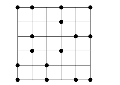
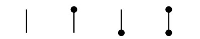
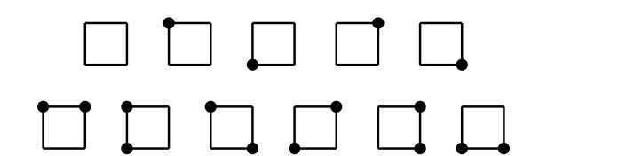
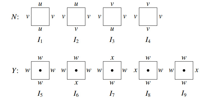
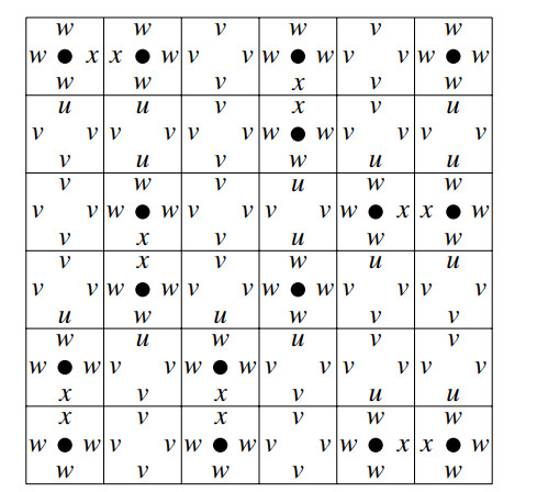
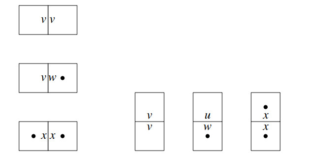
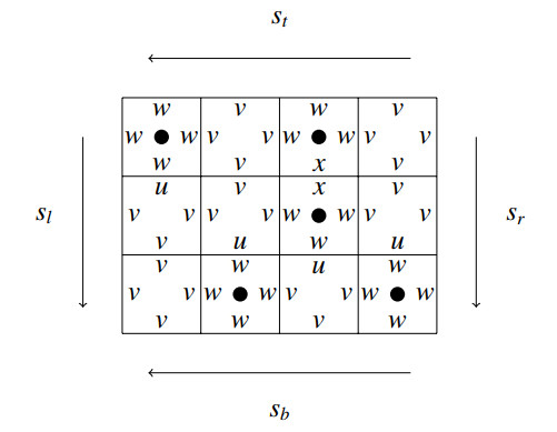
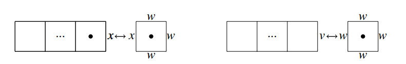
A dissociation set of a graph $ G $ refers to a set of vertices inducing a subgraph with maximum degree at most 1 and serves as a generalization of two fundamental concepts in graph theory: Independent sets and induced matchings. The enumeration of specific substructures in grid graphs has been a captivating area of research in graph theory. Over the past few decades, the enumeration problems related to various structures in grid graphs such as Hamiltonian cycles, Hamiltonian paths, independent sets, maximal independent sets, and dominating sets have been deeply studied. In this paper, we enumerated dissociation sets in grid graphs using the state matrix recursion algorithm.
- dissociation sets,
- enumeration,
- grid graphs,
- state matrix recursion algorithm
Citation: Wenke Zhou, Guo Chen, Hongzhi Deng, Jianhua Tu. Enumeration of dissociation sets in grid graphs[J]. AIMS Mathematics, 2024, 9(6): 14899-14912. doi: 10.3934/math.2024721

Related Papers:

Abstract

A dissociation set of a graph $ G $ refers to a set of vertices inducing a subgraph with maximum degree at most 1 and serves as a generalization of two fundamental concepts in graph theory: Independent sets and induced matchings. The enumeration of specific substructures in grid graphs has been a captivating area of research in graph theory. Over the past few decades, the enumeration problems related to various structures in grid graphs such as Hamiltonian cycles, Hamiltonian paths, independent sets, maximal independent sets, and dominating sets have been deeply studied. In this paper, we enumerated dissociation sets in grid graphs using the state matrix recursion algorithm.

References

[1]	F. Bock, J. Pardey, L. D. Penso, D. Rautenbach, A bound on the dissociation number, J. Graph Theory, 103 (2023), 661–673. https://doi.org/10.1002/jgt.22940 doi: 10.1002/jgt.22940
[2]	F. Bock, J. Pardey, L. D. Penso, D. Rautenbach, Relating the independence number and the dissociation number, J. Graph Theory, 104 (2023), 320–340. https://doi.org/10.1002/jgt.22965 doi: 10.1002/jgt.22965
[3]	N. J. Calkin, H. S. Wilf, The number of independent sets in a grid graph, SIAM J. Discrete Math., 11 (1998), 54–60. https://doi.org/10.1137/S089548019528993X doi: 10.1137/S089548019528993X
[4]	S. Cheng, B. Wu, Number of maximal 2-component independent sets in forests, AIMS Math., 7 (2023), 13537–13562. https://doi.org/10.3934/math.2022748 doi: 10.3934/math.2022748
[5]	A. Itai, C. H. Papadimitriou, J. L. Szwarcfiter, Hamilton paths in grid graphs, SIAM. J. Comput., 11 (1982), 676–686. https://doi.org/10.1137/0211056 doi: 10.1137/0211056
[6]	F. Kardoš, J. Katrenič, I. Schiermeyer, On computing the minimum 3-path vertex cover and dissociation number of graphs, Theoret. Comput. Sci., 412 (2011), 7009–7017. https://doi.org/10.1016/j.tcs.2011.09.009 doi: 10.1016/j.tcs.2011.09.009
[7]	S. Lomonaco, L. Kauffman, Quantum knots, Proc. SPIE, 5436 (2004), 268–284. https://doi.org/10.1117/12.544072
[8]	S. Lomonaco, L. Kauffman, Quantum knots and mosaics, Quantum Inform. Process., 7 (2008), 85–115. https://doi.org/10.1007/s11128-008-0076-7
[9]	S. Oh, State matrix recursion method and monomer-dimer problem, Discrete Math., 342 (2019), 1434–1445. https://doi.org/10.1016/j.disc.2019.01.022 doi: 10.1016/j.disc.2019.01.022
[10]	S. Oh, Number of dominating sets in cylindric square grid graphs, Graphs Combin., 37 (2021), 1357–1372. https://doi.org/10.1007/s00373-021-02323-8 doi: 10.1007/s00373-021-02323-8
[11]	S. Oh, S. Lee, Enumerating independent vertex sets in grid graphs, Linear Alg. Appl., 510 (2016), 192–204. https://doi.org/10.1016/j.laa.2016.08.025 doi: 10.1016/j.laa.2016.08.025
[12]	Y. Orlovich, A. Dolgui, G. Finke, V. Gordon, F. Werner, The complexity of dissociation set problems in graphs, Discrete Appl. Math., 159 (2011), 1352–1366. https://doi.org/10.1016/j.dam.2011.04.023 doi: 10.1016/j.dam.2011.04.023
[13]	W. Sun, S. Li, On the maximal number of maximum dissociation sets in forests with fixed order and dissociation number, Taiwanese J. Math., 27 (2023), 647–683. https://doi.org/10.11650/tjm/230204 doi: 10.11650/tjm/230204
[14]	G. L. Thompson, Hamiltonian tours and paths in rectangular lattice graphs, Math. Mag., 50 (1977), 147–150. https://doi.org/10.1080/0025570X.1977.11976635 doi: 10.1080/0025570X.1977.11976635
[15]	J. Tu, Z. Zhang, Y. Shi, The maximum number of maximum dissociation sets in trees, J. Graph Theory, 96 (2021), 472–489. https://doi.org/10.1002/jgt.22627 doi: 10.1002/jgt.22627
[16]	M. Xiao, S. Kou, Exact algorithms for the maximum dissociation set and minimum 3-path vertex cover problems, Theoret. Comput. Sci., 657 (2017), 86–97. https://doi.org/10.1016/j.tcs.2016.04.043 doi: 10.1016/j.tcs.2016.04.043
[17]	M. Yannakakis, Node-deletion problems on bipartite graphs, SIAM J. Comput., 10 (1981), 310–327. https://doi.org/10.1137/0210022 doi: 10.1137/0210022
[18]	L. Zhang, J. Tu, C. Xin, Maximum dissociation sets in subcubic trees, J. Comb. Optim., 46 (2023), 8. https://doi.org/10.1007/s10878-023-01076-9 doi: 10.1007/s10878-023-01076-9

Reader Comments

Your name:*

Email:*
© 2024 the Author(s), licensee AIMS Press. This is an open access article distributed under the terms of the Creative Commons Attribution License (http://creativecommons.org/licenses/by/4.0)