
Bézier curves are essential for data interpolation. However, traditional Bézier curves often fail to detect special features that may exist in a data set, such as monotonicity or convexity, leading to invalid interpolations. This study aims to improve the deficiency of Bézier curves by imposing monotonicity or convexity-preserving conditions on the shape parameter and control points. For this purpose, the quintic trigonometric Bézier curves with two shape parameters are used. These techniques constrain only one of the shape parameters, leaving the other free to provide users with more freedom and flexibility in modifying the final curve. To guarantee smooth interpolation, the curvature profiles of the curves are analyzed, which aids in selecting the optimal shape parameter values. The effectiveness of the developed schemes was evaluated by implementing real-life data and data obtained from the existing schemes. Compared with the existing schemes, the developed schemes produce low-curvature interpolation curves with unnoticeable wiggles and turns. The proposed methods also work effectively for both nonuniformly spaced data and negative-valued convex data in real-life applications. When the shape parameter is correctly chosen, the developed interpolants exhibit continuous curvature plots, assuring C2 continuity.
Citation: Salwa Syazwani Mahzir, Md Yushalify Misro, Kenjiro T. Miura. Preserving monotone or convex data using quintic trigonometric Bézier curves[J]. AIMS Mathematics, 2024, 9(3): 5971-5994. doi: 10.3934/math.2024292
[1] | Salwa Syazwani Mahzir, Md Yushalify Misro . Enhancing curve smoothness with whale optimization algorithm in positivity and monotonicity-preserving interpolation. AIMS Mathematics, 2025, 10(3): 6910-6933. doi: 10.3934/math.2025316 |
[2] | Pakeeza Ashraf, Ghulam Mustafa, Husna A. Khan, Dumitru Baleanu, Abdul Ghaffar, Kottakkaran Sooppy Nisar . A shape-preserving variant of Lane-Riesenfeld algorithm. AIMS Mathematics, 2021, 6(3): 2152-2170. doi: 10.3934/math.2021131 |
[3] | Noor Adilla Harim, Samsul Ariffin Abdul Karim, Mahmod Othman, Azizan Saaban, Abdul Ghaffar, Kottakkaran Sooppy Nisar, Dumitru Baleanu . Positivity preserving interpolation by using rational quartic spline. AIMS Mathematics, 2020, 5(4): 3762-3782. doi: 10.3934/math.2020244 |
[4] | Samia BiBi, Md Yushalify Misro, Muhammad Abbas . Smooth path planning via cubic GHT-Bézier spiral curves based on shortest distance, bending energy and curvature variation energy. AIMS Mathematics, 2021, 6(8): 8625-8641. doi: 10.3934/math.2021501 |
[5] | Syed Ahmad Aidil Adha Said Mad Zain, Md Yushalify Misro . A novel technique on flexibility and adjustability of generalized fractional Bézier surface patch. AIMS Mathematics, 2023, 8(1): 550-589. doi: 10.3934/math.2023026 |
[6] | Zhiqian He, Man Xu, Yanzhong Zhao, Xiaobin Yao . Bifurcation curves of positive solutions for one-dimensional Minkowski curvature problem. AIMS Mathematics, 2022, 7(9): 17001-17018. doi: 10.3934/math.2022934 |
[7] | Atakan Tuğkan Yakut, Alperen Kızılay . On the curve evolution with a new modified orthogonal Saban frame. AIMS Mathematics, 2024, 9(10): 29573-29586. doi: 10.3934/math.20241432 |
[8] | Abdul Majeed, Muhammad Abbas, Amna Abdul Sittar, Md Yushalify Misro, Mohsin Kamran . Airplane designing using Quadratic Trigonometric B-spline with shape parameters. AIMS Mathematics, 2021, 6(7): 7669-7683. doi: 10.3934/math.2021445 |
[9] | Fengyi Chen . A new GM2(2,1) model based on a C1 convexity-preserving rational quadratic interpolation spline. AIMS Mathematics, 2024, 9(7): 17917-17931. doi: 10.3934/math.2024872 |
[10] | Yating Zhu, Zixun Zeng, Zhong Chen, Deqiang Zhou, Jian Zou . Performance analysis of the convex non-convex total variation denoising model. AIMS Mathematics, 2024, 9(10): 29031-29052. doi: 10.3934/math.20241409 |
Bézier curves are essential for data interpolation. However, traditional Bézier curves often fail to detect special features that may exist in a data set, such as monotonicity or convexity, leading to invalid interpolations. This study aims to improve the deficiency of Bézier curves by imposing monotonicity or convexity-preserving conditions on the shape parameter and control points. For this purpose, the quintic trigonometric Bézier curves with two shape parameters are used. These techniques constrain only one of the shape parameters, leaving the other free to provide users with more freedom and flexibility in modifying the final curve. To guarantee smooth interpolation, the curvature profiles of the curves are analyzed, which aids in selecting the optimal shape parameter values. The effectiveness of the developed schemes was evaluated by implementing real-life data and data obtained from the existing schemes. Compared with the existing schemes, the developed schemes produce low-curvature interpolation curves with unnoticeable wiggles and turns. The proposed methods also work effectively for both nonuniformly spaced data and negative-valued convex data in real-life applications. When the shape parameter is correctly chosen, the developed interpolants exhibit continuous curvature plots, assuring C2 continuity.
Shape-preserving interpolation is a fundamental concept in numerical analysis and data approximations. It is essential for maintaining the important characteristics of a dataset while generating a continuous function that smoothly connects all data points. Monotone data, such as the uric acid level in gout patients [1] and the rate of radioactive decay [2], exhibits a consistent directional trend, either increasing or decreasing, whereas convex data shows a curve that slopes upward. The problem of convex data arises in the design of telecommunication systems, parameter estimation, and approximation theory [3]. Preserving monotonicity and convexity ensures that the interpolated function accurately represents the fundamental behavior of the original data. This field has been revolutionized over the years, improving the way data is interpolated.
The study of monotonicity preservation by [4] proposed a monotonicity-preserving technique using a C1-weighted quadratic spline. As the developed technique is non-rational, it is easy to implement and requires less computational time. [5] presented a monotonicity-preserving technique that achieved GC1 continuity by employing a rational quartic over linear spline function. [6,7] implemented cubic over linear and quadratic rational functions, resulting in C2 interpolant with the unknown derivative values determined by solving a system of tridiagonal equations. [8,9] constructed C1 monotonicity-preserving schemes using (cubic/cubic) and (cubic/quadratic) rational cubic Ball interpolation functions. By having more free parameters, [9] provided greater flexibility for users to modify the resulting curves. On the other hand, [8,10] provided curvature profile comparisons to quantitatively analyze the smoothness of the resulting curves. This approach eliminates the potential biases that may arise from subjective human judgment, providing a more reliable assessment of the curves' smoothness.
Further, subdivision schemes are also common in shape-preserving interpolation due to their ease of use and flexibility. [11] and [12] employed ternary and four-point ternary nonstationary interpolating subdivision schemes for monotonicity-preserving schemes. Furthermore, fractal splines are employed in monotonicity-preserving interpolation. [13,14] created monotonicity-preserving interpolation algorithms based on a rational cubic fractal spline. These schemes involve the scaling and shape parameters. The latter scheme is more flexible because it sets limits only on the shape parameters, thereby leaving the scaling factor free for curve adjustment.
A C1 convexity-preserving piecewise variable-degree rational interpolation spline with two local shape parameters was developed by [15]. Due to the positive second derivatives of the interpolant, the convex data can be directly preserved. Rational cubic and quartic interpolants were used by [16,17,18]. A C1 continuous convexity preserving scheme was developed by [16], whereas [17,18] developed C2 continuous schemes. [17] used LU decomposition to solve for the derivative values, while [18] offered a simpler approach that yields a local scheme by directly computing the derivative values. [19] implemented a trigonometric function with a shape parameter. This approach is rigid because the shape parameter is constrained to preserve convexity. [20] suggested convexity-preserving methods for generalized cubic spline, including rational, exponential, variable power, hyperbolic, and spline with additional knots. The non-convex curve segments are adjusted with near-optimal tension parameters. The developed scheme is universal and can be applied to any type of generalized spline with tension parameters.
First introduced in 1958, Bézier curves have gotten considerable attention due to their simple development and ease of control due to their convex hull properties. In addition, no advanced knowledge of computer aided geometric design (CAGD) is needed to use the curves because they are made up of control points and Bernstein polynomials, which can be easily developed. In addition to the conventional Bézier curve, trigonometric Bézier curves with shape parameters have been proposed [21,22,23], resulting in greater adjustability and control of the curve shape. Because of the nice properties they hold, Bézier curves have been applied to many real-life applications, including highway design [24], path planning [25], image compression [26], and surface construction [27]. However, when applied to data interpolations, Bézier curves neglect important features of the data, resulting in misleading interpolation. This study aims to incorporate the shape-preserving approach into the trigonometric Bézier curves by developing data-dependent constraints on the shape parameter and introducing a scaling factor on the control points to ensure the control points' monotonicity or convexity. Curvature analysis is also conducted to assess the smoothness of the resulting interpolation.
This paper is structured as follows: In Section 2, the C2 quintic trigonometric Bézier interpolating curve is constructed, and the method for computing the derivative values is explained. Next, the derivation of the monotonicity or convexity-preserving conditions for the shape parameter is presented in Section 3. The formula for computing the curvature profile is described in Section 4. Section 5 presents graphical examples of shape-preserving interpolations by implementing new and previous data sets from the existing scheme. Finally, Section 6 provides the conclusion and a few possible directions for further research.
For the purpose of this study, the quintic trigonometric Bézier curve with two shape parameters proposed by [23] will be used. Let {(xi,yi):i=0,1,2,…,n} be a set of data defined over the interval [x0,xn] with xi+1>xi. The quintic trigonometric Bézier curve in each subinterval Ii=[xi,xi+1] is given by
s(x)≡si(x)=5∑j=0Bjfj(x), | (2.1) |
where Bj and fj(x) denote the control points and the basis functions of the quintic trigonometric Bézier curves that are given as follows:
f0(x)=(1−sinθ)4(1−αsinθ),f1(x)=sinθ(1−sinθ)3(4+α−αsinθ),f2(x)=(1−sinθ)2(1−cosθ)(8sinθ+3cosθ+9),f3(x)=(1−cosθ)2(1−sinθ)(8cosθ+3sinθ+9),f4(x)=cosθ(1−cosθ)3(4+β−βcosθ),f5(x)=(1−cosθ)4(1−βcosθ), | (2.2) |
where θ=π(x−xi)2hi with θ∈[0,π2]. The shape parameters α,β∈[−4,1] are responsible for controlling the shape of the curve. The quintic trigonometric Bézier basis functions, fj(x) for j=0,1,2,3,4,5 in Eq (2.2), have the following geometric properties:
(1) Non-negativity:
fj(x)≥0 for all x∈[xi,xi+1]. |
(2) Symmetry:
fj(x)=f5−j(xi+1−x) if α=β. |
(3) Partition of unity:
5∑j=0fj(x)=1 for all x∈[xi,xi+1]. |
In addition, the quintic trigonometric Bézier curve in Eq (2.1) also satisfies other properties such as the endpoint terminal, convex hull, symmetry, and geometric invariance, which were further discussed in [23]. The plot of the quintic trigonometric Bézier basis functions for various values of the shape parameters, α and β, is shown in Figure 1 below.
Next, the C2 interpolating conditions (2.3) will be applied to Eq (2.1) to determine the equations of the unknown control points Bj. Let s′ and s″ be the first-order and second-order derivatives of s, and the interpolating conditions are
s(xi)=yi,s(xi+1)=yi+1,s′(xi)=di,s′(xi+1)=di+1,s″(xi)=Di,s″(xi+1)=Di+1, | (2.3) |
where di and Di are the first-order and second-order derivative values at knots.
Taking into account the local variable relative to Ii, from Eqs (2.1)–(2.3) it is straightforward to establish that
B0=yi,B1=yi+2hidi(4+αi)π,B2=yi+hi((4+αi)Dihi+4(3+αi)diπ)3(4+αi)π2,B3=yi+1−hi((βi−4)Di+1hi+4(3+βi)di+1π)3(4+βi)π2,B4=yi+1−2hidi+1(4+βi)π,B5=yi+1, | (2.4) |
with hi=xi+1−xi.
As a result, the C2 quintic trigonometric Bézier curve with two shape parameters in Eq (2.1) defined over each subinterval Ii can be written as
s(x)=5∑j=0Bjfj(x)=yi(1−sinθ)4(1−αisinθ)+(yi+2hidi(4+αi)π)sinθ(1−sinθ)3(4+αi−αisinθ)+(yi+hi((4+αi)Dihi+4(3+αi)diπ)3(4+αi)π2)(1−sinθ)2(1−cosθ)(8sinθ+3cosθ+9)+(yi+1+hi((4+βi)Di+1hi−4(3+βi)di+1π)3(4+βi)π2)(1−cosθ)2(1−sinθ)(8cosθ+3sinθ+9)+(yi+1−2hidi+1(4+βi)π)cosθ(1−cosθ)3(4+βi−βicosθ)+yi+1(1−cosθ)4(1−βicosθ). | (2.5) |
In this research, the values of di and Di are both calculated from the given data using the arithmetic mean method (AMM).
From [28], the first-order derivative values at the first knot are as follows:
d0=Δ0+(Δ0−Δ1)h0h0+h1, | (2.6) |
di=Δi+Δi+12 for i=1,2,…,n−1, | (2.7) |
dn=Δn−1+(Δn−1−Δn−2)hn−1hn−1+hn−2, | (2.8) |
where Δi=yi+1−yihi.
Meanwhile, the second-order derivative values at the first knot are given by the following [28]:
D0=M0+(M0−M1)h0h0+h1, | (2.9) |
Di=Mi+Mi+12 for i=1,2,…,n−1, | (2.10) |
Dn=Mn−1+(Mn−1−Mn−2)hn−1hn−1+hn−2, | (2.11) |
with Mi=di+1−dihi.
The C2 quintic trigonometric Bézier curve constructed in Section 2 does not guarantee data-shape preservation. Therefore, this section will develop shape-preserving constraints, specifically on the shape parameter αi, which controls the left end of the interpolation curves. The shape parameter βi, which controls the right-end part of the curves, will remain flexible to allow modification of the resulting curve according to the user's preference. Moreover, the control points will also be restricted and automatically calculated for shape preservation.
Suppose (xi,yi) is a monotonically increasing data set such that
yi+1≥yi with xi+1≥xi. | (3.1) |
Thus, it is straightforward to establish that Δi≥0 and di≥0.
Theorem 3.1. The C2 quintic trigonometric Bézier curves defined in Eq (2.5) will preserve the monotonicity of monotone data if the parameters αi, βi, ¯hi, and ¯h∗i in each subinterval satisfy the following conditions:
βi∈(−4,1], which produces a monotone curve, and αi∈[li,ui] for
li=min{0,−2hidiπyi−4,4πhidi3π2yi+4πdihi+Dih2i−4}, | (3.2) |
ui=max{1,−2hidiπyi,4πhidi3π2yi+4πdihi+Dih2i}. | (3.3) |
Let bjforj=1,2,3,4 be the second terms in Bj
{¯hi=hiki,ifb1>dyi2orb2>dyi2,¯h∗i=hik∗i,ifb3>dyi2orb4>dyi2,¯hi=¯h∗i=hi,elsewhere, | (3.4) |
where ki,k∗i satisfy Eqs (3.9) and (3.10).
Proof. The C2 quintic trigonometric Bézier curves (2.5) will preserve the monotonicity of data if
s(1)(x)≥0. |
Differentiating s(x) with respect to x results in 16 terms that are associated with both shape parameters αi and βi. As this study aims to constrain only the shape parameter αi, only eight terms that are associated with the shape parameter, αi, are considered, as given by the following equation:
s(1)α(x)=7∑j=0Ajkj(x)≥0, | (3.5) |
where kj(x) for j=0,1,2,…,7 are non-negative functions defined in Eq (3.6). The plot of the functions is demonstrated in Figure 2.
k0(x)=cosθ(1−sinθ)4,k1(x)=cosθsinθ(1−sinθ)3,k2(x)=(1−cosθ)cosθ(1−sinθ)(9+3cosθ+8sinθ),k3(x)=(1−sinθ)2sinθ(9+3cosθ+8sinθ),k4(x)=(1−cosθ)(1−sinθ)2(8cosθ−3sinθ),k5(x)=cosθ(1−sinθ)3(1−αsinθ),k6(x)=cosθ(1−sinθ)3(4+α−αsinθ),k7(x)=cosθ(1−sinθ)2sinθ(4+α−αsinθ). | (3.6) |
Since kj(x) is already greater than zero, mathematical derivations are needed to ensure Aj≥0 for j=0,1,2,…,7, hence, guaranteeing Eq (3.5). This will be done by letting Aj≥0 and solving for αi.
(1) Let A0=−αiπyi2hi≥0. Solving in terms of αi results in αi≤0.
(2) A1=−αiπ(yi+2dihi(4+αi)π)2hi≥0. Simplified and rearranged, this yields αi≤−2hidπyi−4.
(3) For A2=−π(yi+hi(4π(3+αi)di+(4+αi)hiDi)3π2(4+αi))hi≥0, solving for αi gives αi≤4πhidih2iDi+4πhidi+3π2yi−4.
(4) Then, A3=A4. Letting these terms be greater than zero produces A3=A4= π(yi+hi(4π(3+αi)di+(4+αi)hiDi)3π2(4+αi))2hi≥0. Rearrangement and simplifications result in αi≥4πhidih2iDi+4πhidi+3π2yi−4, which acts as a lower bound for monotonicity preservation and can be simplified as αi≥4πhidih2iDi+4πhidi+3π2yi. (5) A5=2πyihi is already greater than zero.
(6) Let A6≥0, giving A6=π(yi+2hidi(4+αi)π)2hi≥0. Next, solving in terms of αi produces αi≤−2hidπyi−4.
(7) Lastly, for A7=−3π(yi+2hidi(4+αi)π)2hi≥0, solving for αi yields αi≥−2hidπyi−4, which acts as the lower bound. This, can be simplified to αi≥−2hidπyi.
To summarize, the constraints for αi above can be written as:
αi≤−2hidπyi−4,αi≤4πhidih2iDi+4πhidi+3π2yi−4,αi≤0,αi≥−2hidπyi,αi≥4πhidih2iDi+4πhidi+3π2yi, | (3.7) |
which can be rearranged as below:
li=min{−2hidiπyi−4,4πhidih2iDi+4πhidi+3π2yi−4,0},ui=max{−2hidiπyi,4πhidih2iDi+4πhidi+3π2yi},ui≤αi≤li. | (3.8) |
Moreover, to ensure a monotonically increasing interpolation, the control points Bj for j = 0,1,2,3,4,5 also need to be monotonically increasing. For this purpose, new conditions for the control points will be developed. Let the second term in the control points Bj for j=1,2,3,4 be bj and dyi=yi+1−yi be the vertical difference between two neighboring data points.
If b1 or b2>dyi2, the control points B1 and B2 from Eq (2.4) will be greater than B5. Since B5=yi+1, this will cause the interpolating curve to rise and drop, resulting in oscillation. Thus, to avoid this, a scaling factor will be introduced by replacing hi in b1 and b2 with ¯hi=hiki, where
ki>max{4πhidi(4+αi)πdyi,4(3+αi)hidi+√2h2i(8(3+αi)2d2i+3(4+αi)2Didyi)3(4+αi)πdyi}. | (3.9) |
These constraints are developed by letting b1 and b2<dyi2. Similarly, if b3 or b4>dyi2, new scaling factor ¯h∗i=hik∗i will be developed by assuming b3 and b4<dyi2 such that
k∗i>max{4πhidi+1(4+βi)πdyi,4(3+βi)hidi+1+√2h2i(8(3+βi)2d2i+1+3(4+βi)2Di+1dyi)3(4+βi)πdyi}. | (3.10) |
A given data set {(xi,yi):i=0,1,2,…,n} is said to be convex if
Δi+1≥Δi and di+1≥di with di+1≥Δi≥di, | (3.11) |
for i=0,1,2,…,n [19]. Graphically, a convex curve can be verified by connecting any two points on the curve. If none of the lines lie below the curve, then it is convex. Theorem 3.2 presents the convexity-preserving interpolation method.
Theorem 3.2. The C2 quintic trigonometric Bézier curves defined in Eq (2.5) will preserve the convexity of convex data if the parameters αi, βi, ¯hi, and ¯h∗i in each subinterval satisfy the following conditions:
βi∈(−4,1], which produces a smooth and convex curve, and αi∈[li,ui], where
li=−2hidiπyi−4, | (3.12) |
ui=max{0,4πhidih2iDi+4πhidi+3π2yi}. | (3.13) |
Let bj for j=1,2,3,4 be the second terms of Eq (2.4). If di>0,
{¯hi=hiki,ifb1>dyi2orb2>dyi2,¯h∗i=hik∗i,ifb3>dyi2orb4>dyi2,¯hi=¯h∗i=hi,elsewhere, | (3.14) |
where ki,k∗i are defined as (3.9) and (3.10). If di<0,
{¯hi=hiki,ifb1<dyi2orb2<dyi2,¯h∗i=hik∗i,ifb3<dyi2orb4<dyi2,¯hi=¯h∗i=hi,elsewhere, | (3.15) |
for ki,k∗i given in Eqs (3.21) and (3.22).
Proof. The C2 quintic trigonometric Bézier curves will preserve data convexity if
s(2)(x)≥0. | (3.16) |
Second-order differentiation of s(x) with respect to x produces 18 terms associated with shape parameters αi and βi. Similarly, only the terms associated with αi will be considered, as given:
s(2)α(x)=9∑j=0Cjgj(x), | (3.17) |
where gj(x) for j=0,1,2,…,8 are defined as follows:
g0(x)=cos2θ(1−sinθ)3,g1(x)=(1−sinθ)4sinθ,g2(x)=cosθ(1−sinθ)2(9+3cosθ+8sinθ),g3(x)=(4+αi−αisinθ)(6π2cos2θ(1−sinθ)+3π2(1−sinθ)2sinθ),g4(x)=(1−αisinθ)(3π2cos2θ(1−sinθ)2+π2(1−sinθ)3sinθ),g5(x)=12π2(−1+sinθ)sinθ(3+9cos2θ+6sinθ+4cosθ(5+12sinθ)),g6(x)=cosθ(1−sinθ)2(−αiπcosθsinθ+πcosθ(4+αi−αisinθ)),g7(x)=(1−sinθ)3(2αiπ2cos2θ−αiπ2sin2θ+π2sinθ(4+αi−αisinθ)),g8(x)=−π2sin2θ2(−1+sinθ)(44+6cosθ−72cos2θ+88sinθ+27sin2θ). | (3.18) |
Similarly, the functions of gj(x) in Eq (3.18) are greater than or equal to zero. Thus, to guarantee Inequality (3.16) holds, derivations will be made so that Cj for j=0,1,2,…,8 are greater than or equal to zero.
(1) Let C0=2αiπ2yih2i≥0. Solving in terms of αi results in αi≥0.
(2) Similarly, C1=αiπ2yi4h2i≥0 gives αi≥0.
(3) For C2=π2(yi+hi(4π(3+αi)di+(4+αi)hiDi)3π2(4+αi))4h2i≥0, solving for αi produces αi≥4πhidih2iDi+4πhidi+3π2yi.
(4) Next, assume C3=yi+2hidiπ(4+αi4h2i≥0. Simplified and rearranged, this yields αi≤−2dihiπyi−4.
(5) Because the data used is convex, C4=yi is convex.
(6) Let C5=π(yi+hi(4π(3+αi)di+(4+αi)hiDi)3π2(4+αi))2h2i≥0 and solve in terms of αi, which gives αi≥4πhidih2iDi+4πhidi+3π2yi.
(7) Suppose C6=3π(yi+2hidiπ(4+αi))4h2i≥0, and after some rearrangements, this gives αi≤−2hidiπyi−4.
(8) Rearrange C7=−yi+2hidiπ(4+αi)4h2i≥0 in terms of αi, which gives αi≤−2hidiπyi−4.
(9) Finally, let C8=yi+hi(4π(3+αi)di+(4+αi)hiDi)3π2(4+αi)4h2i≥0, and rearranging in terms of αi results in αi≥4πhidih2iDi+4πhidi+3π2yi.
In summary, items (1)–(9) above can be written as:
αi≤−2hidπyi−4,αi≥0,αi≥4πhidih2iDi+4πhidi+3π2yi, | (3.19) |
which can be rearranged to produce the following conditions:
li=−2hidiπyi−4,ui=max{0,4πhidih2iDi+4πhidi+3π2yi},ui≤αi≤li. | (3.20) |
Next, the control points Bj for j=0,1,2,3,4,5 in Eq (2.4) for each subinterval must be set convex. Convex data are allowed to be monotonically increasing or decreasing in an interval. Thus, there are two cases to consider.
For the first case, which involves a monotonically increasing interval, the same conditions as in Eqs (3.9) and (3.10) will be applied. However, for monotone-decreasing interval, slight modifications will be made to the conditions. Suppose the second term in control points Bj for j=1,2,3,4 is bj, and dyi=yi+1−yi is the vertical difference between two neighboring data points. In the monotone decreasing interval, yi+1≤yi. Thus, dyi≤0 and di≤0. Consequently, bj≤0. If b1 or b2<dyi2, or in other words, b1 and b2 are more negative than the half vertical difference, then yi in (2.4) will be added with a number less than the negative vertical difference. Hence, b1 and b2 will be smaller than b5, and the curve will drop and rise, which will produce a non-monotone interval. To prevent this, hi in b1 and b2 will be replaced by ¯hi=hiki, where ki is the scaling factor introduced to ensure b1 and b2>dyi2. Next, ki is defined as follows:
ki>max{4πhidi(4+αi)πdyi,4(3+αi)hidi−√2h2i(8(3+αi)2d2i+3(4+αi)2Didyi)3(4+αi)πdyi}. | (3.21) |
Similarly, if b3 or b4<dyi2, scaling factors ¯h∗i=hik∗i will be developed by assuming b3 and b4>dyi2 such that
k∗i>max{4πhidi+1(4+βi)πdyi,4(3+βi)hidi+1−√2h2i(8(3+βi)2d2i+1+3(4+βi)2Di+1dyi)3(4+βi)πdyi}. | (3.22) |
Figure 3 depicts the flowchart of the proposed method to improve understanding. Algorithm 1 summarizes the method for generating C2 monotonicity or convexity-preserving curves.
Algorithm 1: Monotonicity or convexity-preserving interpolation. |
(1) Input data points {(xi,yi)}ni=0. |
(2) Compute the values of hi=xi+1−xi and Δi=yi+1−yihi. |
(3) Calculate first and second-order derivatives as discussed in Section 2.1. |
(4) For each subinterval Ii, choose any value of βi∈(−4,1]. |
(5) Calculate the values of parameters αi and hi based on Theorems 3.1 and 3.2. |
(6) Construct the C2 quintic trigonometric Bézier interpolating curve defined in (2.5) using the accumulated values obtained in Steps 1 to 5. |
To ensure visually pleasing curves, this study implemented two ways of choosing the optimal βi values: visual comparison and curvature analysis. For curvature analysis, the following formulation will be used to determine the smoothness. Let s(x)=(sx(x),sy(x)) be a 2D parametric curve of s(x). The curvature of the curve, κ, is defined as follows:
κ(x)=|s′(x)×s″(x)||s′(x)|3, | (4.1) |
which can also be expressed as
κ(x)=s′x(x)s″y(x)−s″x(x)s′y(x)[s′x(x)2+s′y(x)2]3/2, | (4.2) |
where s′x(x) and s″x(x) are the first and second-order partial derivatives of x. Meanwhile, s′y(x) and s″y(x) are the partial derivatives of y with respect to x.
In this section, numerical experiments were conducted using MATLAB Software to assess the efficiency of the developed methods. Newly proposed data sets as well as data sets taken from the existing schemes were implemented for comparisons and validation.
Example 5.1. Table 1 depicts a random monotone data set taken from [5].
Example 5.2. Table 2 provides an experimental data set of an electronic circuit's waveform distortion taken from [7]. The data demonstrated monotone increasing behavior with the x-values representing the voltage (V), while the y-values are the current (A).
i | 1 | 2 | 3 | 4 | 5 | 6 | 7 | 8 | 9 | 10 | 11 |
xi | 0 | 2 | 3 | 5 | 6 | 8 | 9 | 11 | 12 | 14 | 15 |
yi | 10 | 10 | 10 | 10 | 10 | 10 | 10.5 | 15 | 50 | 60 | 85 |
Figures 4 and 5 show the interpolation of monotone data from Tables 1 and 2, respectively. Figures 4a and 5a show the interpolation curves using the traditional C2 quintic trigonometric Bézier curves without satisfying the monotonicity-preserving constraints, where the shape parameters, αi and βi, in each subinterval, are set to 0.5. The interpolation curves fail to retain the monotonicity of the data, which can be observed in the third subinterval of Figure 4a as well as the seventh and ninth subintervals of Figure 5a. Figures 4b and 5b demonstrate the monotonicity preserving interpolation curves with the shape parameter αi satisfying Theorem 3.1 for several βi values within the interval (−4,1]. The goal is to observe the best βi values that give the smoothest interpolating curves.
From Figure 4b, it can be observed that all βi values in the first subinterval produced similar interpolation curves. This is because the shape parameter βi is associated with the right end of the curve. As the second subinterval is constant, the values of the first- and second-order derivatives are both zero. Consequently, changes in the shape parameter did not affect the last three control points of the subinterval. βi=−3.5 and βi=−2.5 in the third subinterval produce oscillating interpolations. Hence, this value must be avoided in the subinterval. By further examining the interpolation curves with varying values of βi, the values of βi∈[−1.5,0.5] are preferable because they produce a more visually pleasing interpolation. This can be proven using a curvature comparison, as shown in Figure 4c.
The curvature plots for βi∈[−1.5,0.5] have the lowest amplitude, indicating the smoothest curve. The interpolating curve with the optimal βi values is shown in Figure 4c. Although βi=0,0.5 have the lowest curvature for x∈[22,30], they result in a sharper curve than βi=−1.5 because the low-curvature curve produces a straight curve towards the next data point. Thus, βi=−1.5 in the third subinterval is the optimal value. As for the last subinterval, a sharp turn is observed at the joint due to the sudden increase in the data point over a small range of data. Despite this, the continuity of the curvature plot is still maintained, as shown in Figure 4d, confirming C2 continuity.
For Example 5.2, flat data points are observed for subintervals i=1,2,3,…,6 of Figure 5b. Hence, constant interpolation curves are obtained. The effect of applying different βi values can be seen starting from the seventh subinterval onwards. Figure 5c illustrates the curvature plots of these subintervals with the vertical orange lines in the figure representing the partitions of the subintervals. βi∈[−1.5,0.5] exhibits low curvature for the subintervals; hence, these values can be chosen. Figure 5d reflects the resulting monotonicity-preserving curves.
The developed method produced comparable interpolation with the existing scheme, as shown in Figure 4f. Further, compared to [7] in Figure 5e, the proposed method produced a smoother curve that increases gradually on the tenth subinterval.
Example 5.3. Table 3 shows the cumulative rainfall data obtained from the Malaysian Meteorological Department, Ministry of Natural Resources, Environment and Climate Change. The data were taken at Bayan Lepas Station for 12 consecutive days from May 26 to June 6, 2022. The days are represented as x-values, whereas the y-values indicate the cumulative amount of rainfall measured in mm3. Due to the non-negativity properties of the rainfall data, this data set is increasing monotonically.
i | 1 | 2 | 3 | 4 | 5 | 6 | 7 | 8 | 9 | 10 | 11 | 12 |
xi | 1 | 2 | 3 | 4 | 5 | 6 | 7 | 8 | 9 | 10 | 11 | 12 |
yi | 1.8 | 3.2 | 3.2 | 3.2 | 11.6 | 16.6 | 48.2 | 67 | 68.4 | 90.8 | 92.8 | 92.9 |
Figure 6a interpolates the data set in Table 3 using the C2 quintic trigonometric Bézier curves with αi=βi=0.5. Despite the monotonicity of the data, the interpolation curves in the fifth, eighth, and tenth subintervals exhibit fluctuations. These fluctuations are due to the large difference and sudden change in the y-values of the i−1 and i subintervals.
Figure 6b illustrates the monotonicity-preserving interpolation with various values of the shape parameter βi, while Figure 6c shows their curvature plots. Figure 6d shows the monotonicity-preserving interpolation with the best values of βi that produce the most visually appealing curve with low curvature.
This data set has uniformly spaced x-values and inconsistent steepness of the y-values, making it different from the previous examples. Therefore, the proposed monotonicity-preserving method is efficient for both uniformly and nonuniformly spaced data points. Furthermore, the monotonicity of the data set is still preserved despite the large differences in the steepness of the data points.
Example 5.4. Table 4 shows a convex data set taken from [19].
Example 5.5. Table 5 shows a data set generated by a convex function f(x)=10/x2 taken from [16].
Figures 7 and 8 present the interpolation curves for the convex data in Tables 4 and 5, respectively.
Figures 7a and 8a demonstrate the failure of the C2 quintic trigonometric Bézier curve to retain data convexity. As shown in the figures, the dotted blue lines connecting the two arbitrarily chosen points on the curves are below the curves. This contradicts the definition of convex curves.
Figures 7b and 8b show the convexity-preserving interpolations with several βi values. βi = −3.5,−2.5 in the third subinterval of Figure 7b result in non-convex interpolation. Moreover, from the curvature plot in Figure 7c, the values of βi in the second subinterval produced disconnected curvature profiles, indicating failure in maintaining C2 continuity due to the constant data points in the subinterval. Hence, these values of βi must be avoided in both subintervals. βi∈[−1.5,0.5] yielded the lowest curvature. Similarly, Figure 8c shows the curvature plot of the curves in Figure 8b. In Figures 7d and 8d, the curves were altered with the best βi to obtain the smoothest C2 interpolating curves.
Compared with existing schemes, the proposed method produces interpolation curves that are looser and smoother with no wiggle, as observed in the first and last subintervals of Figure 7e. This is because the proposed method uses degree-five interpolation curves with four intermediate control points; hence, it is more flexible and has greater control over the curve. Meanwhile, in Figure 8e, the curve of the proposed method is observed to be tighter, but in the second and fourth subintervals, the developed method displays a steady convex decreasing trend, giving a smooth-looking curve with unnoticeable turning.
Example 5.6. The data of Toyota Prius rooftop measurements taken from [29] are shown in Table 6. The data were measured using a 3D laser scanner, and the data set exhibited a convex shape. In this study, only a subset of the collected data points was used to demonstrate the efficiency of the proposed method.
i | 1 | 2 | 3 | 4 | 5 | 6 | 7 | 8 |
xi | 1848.88 | 1948.09 | 1975.61 | 2516.23 | 2610.93 | 3068.07 | 3100.04 | 3279.18 |
yi | -554.37 | -575.38 | -580.38 | -632.013 | -632.12 | -593.84 | -588.17 | -548.09 |
Figure 9a shows the interpolation using the ordinary C2 quintic trigonometric Bézier curves with shape parameters αi=βi=0.5. Non-convex interpolation can be seen in the third and fifth subintervals due to the large increment and decrement in the size of the data interval.
Figure 9b illustrates the convexity-preserving interpolation with varying βi values to observe the optimal βi. The resulting curves are analyzed quantitatively using the curvature plot shown in Figure 9c. The optimal βi values are then chosen based on the observation and curvature plot to generate smooth convexity-preserving curves, as shown in Figure 9d. This example demonstrates that the proposed method is effective not only for positively valued convex data but also for negatively valued convex data.
This study established new methods for preserving monotone or convex data. Quintic trigonometric Bézier curves with two shape parameters that control each end of the curve were used. Shape-preserving constraints were developed only on the left-end curves, whereas the right-end curve could be freely altered by users. This study also analyzed the curvature profiles to demonstrate visually pleasing interpolating curves, which improves the previous research by [30] that relied solely on visual comparison.
The proposed methods outperformed the existing schemes by reducing the wiggles and ensuring smooth increasing and decreasing trends, resulting in interpolation with less noticeable turning. Furthermore, the developed methods work well for both uniform and non-uniformly spaced data. The proposed methods also performed well with negative-valued data. Using a higher-degree Bézier curve, both the first- and second-order derivatives can be entirely calculated using the formula, thus reducing the complexity of the previous study. Furthermore, the higher-degree Bézier curve has a greater number of control points, which increases curve control.
However, for constant data points, some values of βi may cause the curvature plot to disconnect in the joint. Therefore, producing an interpolating curve that is not C2 continuous. The basis functions used in this study can be extended to investigate the shape preservation of surfaces.
The authors declare they have not used artificial intelligence (AI) tools in the creation of this article.
This research was supported by the Ministry of Higher Education Malaysia through the Fundamental Grant Scheme (FRGS/1/2023/STG06/USM/03/4) and the School of Mathematical Sciences, Universiti Sains Malaysia. The authors are very grateful to the anonymous referees for their valuable suggestions.
The authors declare that they have no competing interests in this paper.
[1] |
M. Z. Hussain, M. Hussain, Visualization of data preserving monotonicity, Appl. Math. Comput., 190 (2007), 1353–1364. http://dx.doi.org/10.1016/j.amc.2007.02.022 doi: 10.1016/j.amc.2007.02.022
![]() |
[2] |
M. Sarfraz, M. Z. Hussain, M. Hussain, Shape-preserving curve interpolation, Int. J. Comput. Math., 89 (2012), 35–53. http://dx.doi.org/10.1080/00207160.2011.627434 doi: 10.1080/00207160.2011.627434
![]() |
[3] |
M. Hussain, A. Abd Majid, M. Z. Hussain, Convexity-preserving bernstein-bézier quartic scheme, Egypt. Inform. J., 15 (2014), 89–95. http://dx.doi.org/10.1016/j.eij.2014.04.001 doi: 10.1016/j.eij.2014.04.001
![]() |
[4] |
B. Kvasov, Monotone and convex interpolation by weighted quadratic splines, Adv. Computat. Math., 40 (2014), 91–116. http://dx.doi.org/10.1007/s10444-013-9300-9 doi: 10.1007/s10444-013-9300-9
![]() |
[5] |
S. Karim, K. Pang, Monotonicity preserving using gc 1 rational quartic spline, AIP Conf. Proc., 1482 (2012), 26–31. http://dx.doi.org/10.1063/1.4757432 doi: 10.1063/1.4757432
![]() |
[6] | A. Edeo, G. Gofeb, T. Tefera, Shape preserving C2 rational cubic spline interpolation, ASRJETS, 12 (2015), 110–122. |
[7] |
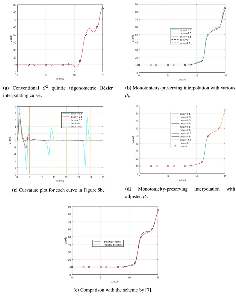
S. Karim, Rational cubic spline interpolation for monotonic interpolating curve with C2 continuity, MATEC Web Conf., 131 (2017), 04016. http://dx.doi.org/10.1051/matecconf/201713104016 doi: 10.1051/matecconf/201713104016
![]() |
[8] | A. Ahmad, M. Misro, Preserving monotonicity of ball curve and it's curvature profile, Proceedings of 6th IEEE International Conference on Recent Advances and Innovations in Engineering (ICRAIE), 2021, 1–6. http://dx.doi.org/10.1109/ICRAIE52900.2021.9704025 |
[9] |
A. Tahat, A. Piah, Z. Yahya, Rational cubic ball curves for monotone data, AIP Conf. Proc., 1750 (2016), 030021. http://dx.doi.org/10.1063/1.4954557 doi: 10.1063/1.4954557
![]() |
[10] | A. Ahmad, M. Misro, Curvature comparison of bézier curve, ball curve and trigonometric curve in preserving the positivity of real data, AMCI, 11 (2022), 12–20. |
[11] |
F. Pitolli, Ternary shape-preserving subdivision schemes, Math. Comput. Simulat., 106 (2014), 185–194. http://dx.doi.org/10.1016/j.matcom.2013.04.003 doi: 10.1016/j.matcom.2013.04.003
![]() |
[12] |
P. Ashraf, M. Sabir, A. Ghaffar, K. Nisar, I. Khan, Shape-preservation of the four-point ternary interpolating non-stationary subdivision scheme, Front. Phys., 7 (2020), 241. http://dx.doi.org/10.3389/fphy.2019.00241 doi: 10.3389/fphy.2019.00241
![]() |
[13] |
A. Chand, N. Vijender, M. Navascués, Shape preservation of scientific data through rational fractal splines, Calcolo, 51 (2014), 329–362. http://dx.doi.org/10.1007/s10092-013-0088-2 doi: 10.1007/s10092-013-0088-2
![]() |
[14] |
P. Viswanathan, A. Chand, A fractal procedure for monotonicity preserving interpolation, Appl. Math. Comput., 247 (2014), 190–204. http://dx.doi.org/10.1016/j.amc.2014.06.090 doi: 10.1016/j.amc.2014.06.090
![]() |
[15] |
L. Peng, Y. Zhu, C1 convexity-preserving piecewise variable degree rational interpolation spline, J. Adv. Mech. Des. Syst., 14 (2020), JAMDSM0002. http://dx.doi.org/10.1299/jamdsm.2020jamdsm0002 doi: 10.1299/jamdsm.2020jamdsm0002
![]() |
[16] |
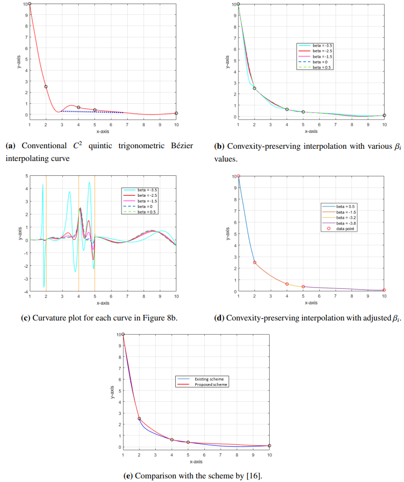
M. Sarfraz, Visualization of positive and convex data by a rational cubic spline interpolation, Inform. Sciences, 146 (2002), 239–254. http://dx.doi.org/10.1016/S0020-0255(02)00209-8 doi: 10.1016/S0020-0255(02)00209-8
![]() |
[17] |
M. Abbas, A. Abd Majid, J. Ali, Local convexity-preserving rational cubic spline for convex data, Sci. World J., 2014 (2014), 391568. http://dx.doi.org/10.1155/2014/391568 doi: 10.1155/2014/391568
![]() |
[18] |
Y. Zhu, C2 rational quartic/cubic spline interpolant with shape constraints, Results Math., 73 (2018), 127. http://dx.doi.org/10.1007/s00025-018-0883-9 doi: 10.1007/s00025-018-0883-9
![]() |
[19] |
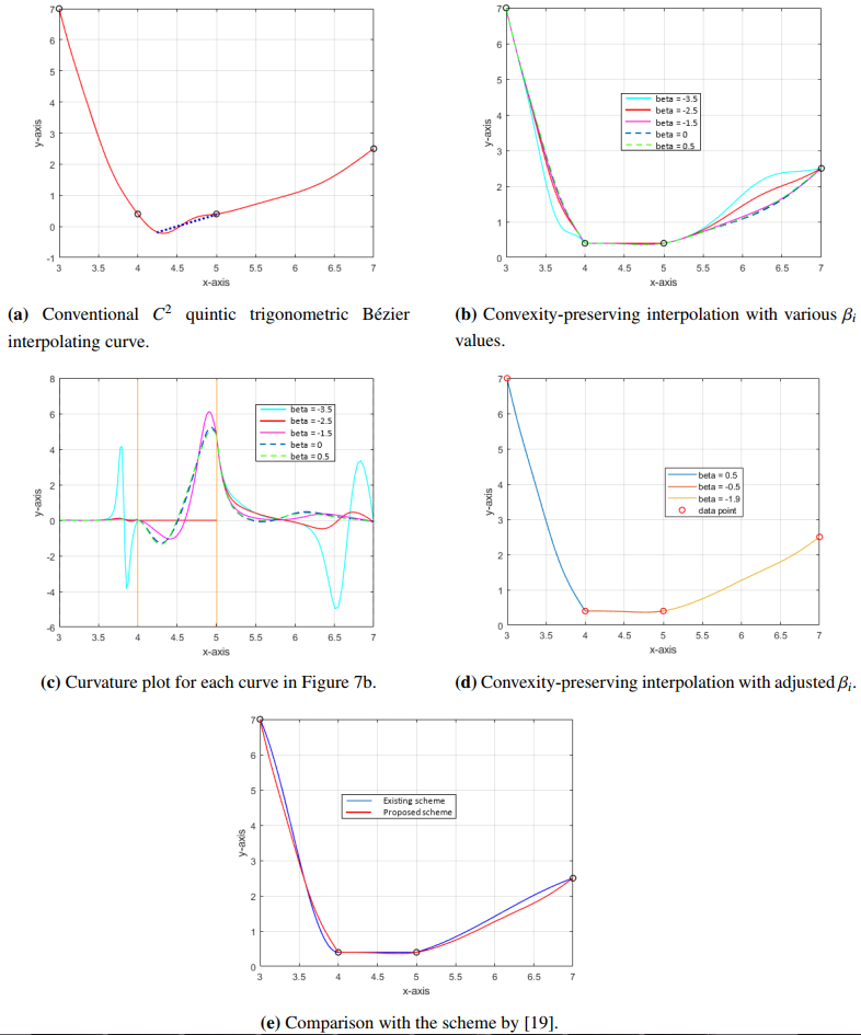
M. Z. Hussain, M. Hussain, A. Waseem, Shape-preserving trigonometric functions, Comp. Appl. Math., 33 (2014), 411–431. http://dx.doi.org/10.1007/s40314-013-0071-1 doi: 10.1007/s40314-013-0071-1
![]() |
[20] |
V. Bogdanov, Y. Volkov, Near-optimal tension parameters in convexity preserving interpolation by generalized cubic splines, Numer. Algor., 86 (2021), 833–861. http://dx.doi.org/10.1007/s11075-020-00914-9 doi: 10.1007/s11075-020-00914-9
![]() |
[21] |
X. Han, Y. Ma, X. Huang, The cubic trigonometric bézier curve with two shape parameters, Appl. Math. Lett., 22 (2009), 226–231. http://dx.doi.org/10.1016/j.aml.2008.03.015 doi: 10.1016/j.aml.2008.03.015
![]() |
[22] |
S. Maqsood, M. Abbas, G. Hu, A. Ramli, K. Miura, A novel generalization of trigonometric bézier curve and surface with shape parameters and its applications, Math. Probl. Eng., 2020 (2020), 4036434. http://dx.doi.org/10.1155/2020/4036434 doi: 10.1155/2020/4036434
![]() |
[23] |
M. Misro, A. Ramli, J. Ali, Quintic trigonometric bézier curve with two shape parameters, Sains Malays., 46 (2017), 825–831. http://dx.doi.org/10.17576/jsm-2017-4605-17 doi: 10.17576/jsm-2017-4605-17
![]() |
[24] |
M. Misro, A. Ramli, J. Ali, Quintic trigonometric bézier curve and its maximum speed estimation on highway designs, AIP Conf. Proc., 1974 (2018), 020089. http://dx.doi.org/10.1063/1.5041620 doi: 10.1063/1.5041620
![]() |
[25] |
V. Bulut, Path planning for autonomous ground vehicles based on quintic trigonometric bézier curve: path planning based on quintic trigonometric bézier curve, J. Braz. Soc. Mech. Sci. Eng., 43 (2021), 104. http://dx.doi.org/10.1007/s40430-021-02826-8 doi: 10.1007/s40430-021-02826-8
![]() |
[26] |
J. Li, D. Zhao, An investigation on image compression using the trigonometric bézier curve with a shape parameter, Math. Probl. Eng., 2013 (2013), 731648. http://dx.doi.org/10.1155/2013/731648 doi: 10.1155/2013/731648
![]() |
[27] |
N. Ismail, M. Misro, Surface construction using continuous trigonometric bézier curve, AIP Conf. Proc., 2266 (2020), 040012. http://dx.doi.org/10.1063/5.0018101 doi: 10.1063/5.0018101
![]() |
[28] |
M. Z. Hussain, M. Hussain, Z. Yameen, A C2-continuous rational quintic interpolation scheme for curve data with shape control, J. Nati. Sci. Found. Sri, 46 (2018), 341–354. http://dx.doi.org/10.4038/jnsfsr.v46i3.8486 doi: 10.4038/jnsfsr.v46i3.8486
![]() |
[29] |
S. Graiff Zurita, K. Kajiwara, K. Miura, Fairing of planar curves to log-aesthetic curves, Japan J. Indust. Appl. Math., 40 (2023), 1203–1219. http://dx.doi.org/10.1007/s13160-023-00567-w doi: 10.1007/s13160-023-00567-w
![]() |
[30] |
S. Mahzir, M. Misro, Shape preserving interpolation of positive and range-restricted data using quintic trigonometric bézier curves, Alex. Eng. J., 80 (2023), 122–133. http://dx.doi.org/10.1016/j.aej.2023.08.009 doi: 10.1016/j.aej.2023.08.009
![]() |
1. | Salwa Syazwani Mahzir, Md Yushalify Misro, Enhancing curve smoothness with whale optimization algorithm in positivity and monotonicity-preserving interpolation, 2025, 10, 2473-6988, 6910, 10.3934/math.2025316 | |
2. | Anis Solehah Mohd Kamarudzaman, Md Yushalify Misro, Kenjiro T. Miura, Feature extraction and analysis of adjustable surfaces in computer graphics, 2025, 37, 1319-1578, 10.1007/s44443-025-00011-8 |
i | 1 | 2 | 3 | 4 | 5 | 6 | 7 | 8 | 9 | 10 | 11 |
xi | 0 | 2 | 3 | 5 | 6 | 8 | 9 | 11 | 12 | 14 | 15 |
yi | 10 | 10 | 10 | 10 | 10 | 10 | 10.5 | 15 | 50 | 60 | 85 |
i | 1 | 2 | 3 | 4 | 5 | 6 | 7 | 8 | 9 | 10 | 11 | 12 |
xi | 1 | 2 | 3 | 4 | 5 | 6 | 7 | 8 | 9 | 10 | 11 | 12 |
yi | 1.8 | 3.2 | 3.2 | 3.2 | 11.6 | 16.6 | 48.2 | 67 | 68.4 | 90.8 | 92.8 | 92.9 |
i | 1 | 2 | 3 | 4 | 5 | 6 | 7 | 8 |
xi | 1848.88 | 1948.09 | 1975.61 | 2516.23 | 2610.93 | 3068.07 | 3100.04 | 3279.18 |
yi | -554.37 | -575.38 | -580.38 | -632.013 | -632.12 | -593.84 | -588.17 | -548.09 |
i | 1 | 2 | 3 | 4 | 5 |
x | 0 | 6 | 10 | 29.5 | 30 |
y | 0.01 | 15 | 15 | 25 | 30 |
i | 1 | 2 | 3 | 4 | 5 | 6 | 7 | 8 | 9 | 10 | 11 |
xi | 0 | 2 | 3 | 5 | 6 | 8 | 9 | 11 | 12 | 14 | 15 |
yi | 10 | 10 | 10 | 10 | 10 | 10 | 10.5 | 15 | 50 | 60 | 85 |
i | 1 | 2 | 3 | 4 | 5 | 6 | 7 | 8 | 9 | 10 | 11 | 12 |
xi | 1 | 2 | 3 | 4 | 5 | 6 | 7 | 8 | 9 | 10 | 11 | 12 |
yi | 1.8 | 3.2 | 3.2 | 3.2 | 11.6 | 16.6 | 48.2 | 67 | 68.4 | 90.8 | 92.8 | 92.9 |
i | 1 | 2 | 3 | 4 |
xi | 3 | 4 | 5 | 7 |
yi | 7 | 0.4 | 0.4 | 2.5 |
i | 1 | 2 | 3 | 4 | 5 |
xi | 1 | 2 | 4 | 5 | 10 |
yi | 10 | 2.5 | 0.625 | 0.4 | 0.1 |
i | 1 | 2 | 3 | 4 | 5 | 6 | 7 | 8 |
xi | 1848.88 | 1948.09 | 1975.61 | 2516.23 | 2610.93 | 3068.07 | 3100.04 | 3279.18 |
yi | -554.37 | -575.38 | -580.38 | -632.013 | -632.12 | -593.84 | -588.17 | -548.09 |