Enhancing structural health monitoring with machine learning for accurate prediction of retrofitting effects

A. Presno Vélez; M. Z. Fernández Muñiz; J. L. Fernández Martínez; A. Presno Vélez; M. Z. Fernández Muñiz; J. L. Fernández Martínez

doi:10.3934/math.20241472

AIMS Mathematics

2024, Volume 9, Issue 11: 30493-30514. doi: 10.3934/math.20241472

Previous Article Next Article

Research article Special Issues

Enhancing structural health monitoring with machine learning for accurate prediction of retrofitting effects

Department of Mathematics, Group of inverse problems, optimization and machine learning, Oviedo University, c/Federico García Lorca 18, Oviedo 33007, Spain

Received: 05 June 2024 Revised: 15 October 2024 Accepted: 23 October 2024 Published: 28 October 2024
MSC : 68T45, 93C95

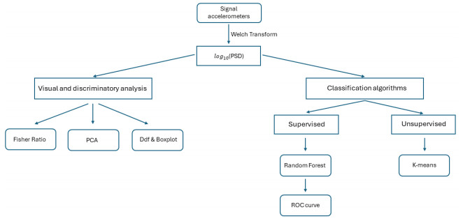
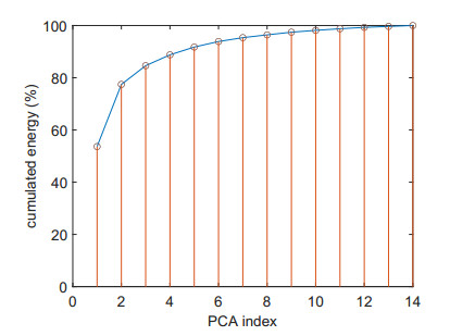
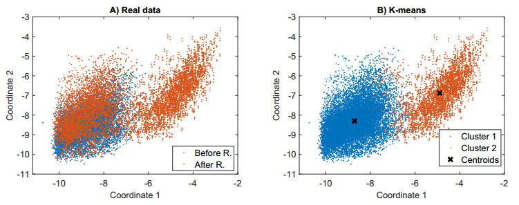
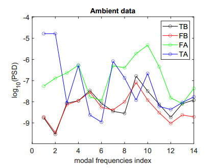
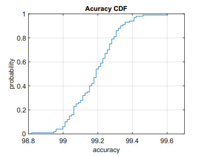
Structural health in civil engineering involved maintaining a structure's integrity and performance over time, resisting loads and environmental effects. Ensuring long-term functionality was vital to prevent accidents, economic losses, and service interruptions. Structural health monitoring (SHM) systems used sensors to detect damage indicators such as vibrations and cracks, which were crucial for predicting service life and planning maintenance. Machine learning (ML) enhanced SHM by analyzing sensor data to identify damage patterns often missed by human analysts. ML models captured complex relationships in data, leading to accurate predictions and early issue detection. This research aimed to develop a methodology for training an artificial intelligence (AI) system to predict the effects of retrofitting on civil structures, using data from the KW51 bridge (Leuven). Dimensionality reduction with the Welch transform identified the first seven modal frequencies as key predictors. Unsupervised principal component analysis (PCA) projections and a K-means algorithm achieved $70 \%$ accuracy in differentiating data before and after retrofitting. A random forest algorithm achieved $99.19 \%$ median accuracy with a nearly perfect receiver operating characteristic (ROC) curve. The final model, tested on the entire dataset, achieved $99.77 \%$ accuracy, demonstrating its effectiveness in predicting retrofitting effects for other civil structures.

Keywords:

Citation: A. Presno Vélez, M. Z. Fernández Muñiz, J. L. Fernández Martínez. Enhancing structural health monitoring with machine learning for accurate prediction of retrofitting effects[J]. AIMS Mathematics, 2024, 9(11): 30493-30514. doi: 10.3934/math.20241472

Related Papers:

[1]	Zongqi Sun, Peng Yang, Ying Wang, Jing Lu . Research on the wealth management fees of defined contribution pensions during the pre-retirement stage. AIMS Mathematics, 2024, 9(12): 36102-36115. doi: 10.3934/math.20241713
[2]	Wanlu Zhang, Hui Meng . Robust optimal investment-reinsurance strategies with the preferred reinsurance level of reinsurer. AIMS Mathematics, 2022, 7(6): 10024-10051. doi: 10.3934/math.2022559
[3]	Xiaoyi Tang, Wei Liu, Wanyin Wu, Yijun Hu . An optimal investment strategy for DC pension plans with costs and the return of premium clauses under the CEV model. AIMS Mathematics, 2024, 9(8): 21731-21754. doi: 10.3934/math.20241057
[4]	Peng Yang . Robust optimal reinsurance-investment problem for $n$ competitive and cooperative insurers under ambiguity aversion. AIMS Mathematics, 2023, 8(10): 25131-25163. doi: 10.3934/math.20231283
[5]	Ling Chen, Xiang Hu, Mi Chen . Optimal investment and reinsurance for the insurer and reinsurer with the joint exponential utility under the CEV model. AIMS Mathematics, 2023, 8(7): 15383-15410. doi: 10.3934/math.2023786
[6]	Yinghui Dong, Chengjin Tang, Chunrong Hua . Optimal investment of DC pension plan under a joint VaR-ES constraint. AIMS Mathematics, 2024, 9(1): 2084-2104. doi: 10.3934/math.2024104
[7]	Wuyuan Jiang, Zechao Miao, Jun Liu . Optimal investment and reinsurance for the insurer and reinsurer with the joint exponential utility. AIMS Mathematics, 2024, 9(12): 35181-35217. doi: 10.3934/math.20241672
[8]	Hui Sun, Zhongyang Sun, Ya Huang . Equilibrium investment and risk control for an insurer with non-Markovian regime-switching and no-shorting constraints. AIMS Mathematics, 2020, 5(6): 6996-7013. doi: 10.3934/math.2020449
[9]	Chunwei Wang, Jiaen Xu, Shujing Wang, Naidan Deng . An investment risk model with bilateral jumps. AIMS Mathematics, 2024, 9(1): 2032-2050. doi: 10.3934/math.2024101
[10]	Jiuchao Ban, Yiran Wang, Bingjie Liu, Hongjun Li . Optimization of venture portfolio based on LSTM and dynamic programming. AIMS Mathematics, 2023, 8(3): 5462-5483. doi: 10.3934/math.2023275

Abstract

Nomenclature

$u, v$	Velocity-components $\left[m.{s}^{-1}\right]$	$S{n}_{x}$	Microorganism density number
$x, y$	Space-coordinate $\left[m\right]$	${N}_{\infty }$	Ambient-microorganism
${B}_{0}$	Magnetic-field strength $\left[N.{m}^{-1}.{A}^{-1}\right]$	${T}_{\infty }$	Ambient-temperature $\left[K\right]$
${U}_{w}\left(x\right)$	Stretching velocity $\left[m.{s}^{-1}\right]$	${C}_{\infty }$	Ambient-concentration
${\left(\rho c\right)}_{p}$	Nanoparticles specific-heat $\left[J.{kg}^{-3}.{K}^{-1}\right]$	${D}_{B}$	Brownian-diffusion coefficient $\left[{m}^{2}.{s}^{-1}\right]$
${\left(\rho c\right)}_{f}$	Thermal capacity of the fluid $\left[J.{kg}^{-3}.{K}^{-1}\right]$	${D}_{m}$	Microorganism-diffusion coefficient $\left[{m}^{2}.{s}^{-1}\right]$
$T$ ${E}_{a}$ ${\sigma }^{**}$ ${\rho }_{p}$	Temperature $\left[K\right]$ Coefficient of activation energy Stefan-Boltzmann constant Density of nanoparticles	${D}_{T}$ $K$ ${k}_{1}$ ${\rho }_{m}$	Thermophoresis-diffusion coefficient $\left[{m}^{2}.{s}^{-1}\right]$ Thermal conductivity Mean-absorption coefficient Microorganism density
${J}_{0}$ ${h}_{f}$ ${M}_{0}$	Density of the current for electrodes Coefficient of heat transfer Magnetization of the permanent magnets of Riga plate	$\nu$ $c$ $a$	Kinematic-viscosity $\left[{m}^{2}.{s}^{-1}\right]$ Stretching rate Distance across the magnets electrodes of Riga plate
$Nc$	Bioconvective Rayleigh-number	$b$	Chemotaxis-constant $\left[m\right]$
$Nr$	Buoyancy-ratio number	$n$	Fitted-rate constant
$Nb$	Brownian-movement number	$\Omega$	Microorganism-difference number
${B}^{*}$	Mixed-convective parameter	$\sigma$	Electrical conductivity $\left[S.{m}^{-1}\right]$
$Nt$	Thermophoretic parameter	$\alpha$	Thermal-diffusivity $\left[{m}^{2}.{s}^{-1}\right]$
$E$	Activation-energy number	${\sigma }^{*}$	Chemical-reaction number
$Le$	Lewis parameter	${W}_{c}$	Cell-swimming-speed $\left[m.{s}^{-1}\right]$
$We$	Weissenberg parameter	$\rho$	Density $\left[kg.{m}^{-3}\right]$
$Pe$	Peclet-parameter	${N}_{w}$	Microorganism at wall
$Lb$	Bioconvective Lewis parameter	${T}_{f}$	Hot fluid temperature $\left[K\right]$
$N{u}_{x}$	Nusselt number	$N$	Microorganism
${C}_{f}$	Skin friction	$K{r}^{2}$	Chemical-reaction-constant
$S{u}_{x}$ $\beta$ $\delta$ $Bi$ $Pr$	Sherwood number Dimensionless parameter Heat generation/absorption parameter Thermal-Biot number Prandtl number	$M$ $S$ $Q$ $Rd$ ${\delta }_{0}$	Magnetic parameter Velocity ratio number Modified Hartmann number Thermal radiation parameter Temperature-difference number

1. Introduction

The description of non-Newtonian fluids has fascinated the interest of various authors due to their wide variety of practical uses in various fields. Walter's B liquid is subclass of non-Newtonian liquids with several manufacturing process applications in industry sectors such as chemical science, biosystems, biophysical techniques of thermal conduction in tissues, chemical manufacturing, and bioengineering. Walters ^[1] was a pioneer of the Walters'-B liquid relation. Nandepanavar et al. ^[2] discussed the impact of nanomaterials in Walters'-B liquid. The effect of nanoparticles in the Walters-B fluid was investigated by Nadeem et al. ^[3]. The effect of the radiative-Walters-B liquid flow and stretched wedge was investigated by Hayat et al. ^[4]. In addition, several scientists have applied the Walters-B relation, which shows the phenomenon of different polymer flows (see ^{[5,6,7,8,9,10]}).

A nanofluid is a fluid that consists of a base fluid with nanosized particles (1–100 nm) suspended in it. Thus, Choi and Eastman ^[11] discussed the fundamental idea of nanomaterials with enhanced thermophysical aspects. Buongiorno ^[12] explained seven-slipping procedures in the movement of nanomaterials, including thermophoresis and Brownian diffusion. Mixed convective nanoliquid transport with the impact of a magnetic field was observed by Hsiao ^[13]. Rashidi et al. ^[14] numerically premeditated the convection characteristics of a nanoliquid through a nonlinear isothermal stretching sheet. Sheikholeslami and Bhatti ^[15] identified the impact of nanomaterials on the transport of nanoliquids via forced-convection through gravitational-force. Turkyilmazoglu ^[16] analyzed nanomaterial transport by vertical surfaces. Ellahi et al. ^[17] noted Jeffrey MHD nanoliquid motion between two parallel-disks. Pantokratoras et al. ^[18] discussed mixed convective fluids with nanoparticles. Rashid et al. ^[19] deliberated the behavior of activation energy in the MHD flow of Maxwell nanoliquid. Tayebi et al. ^[20] explored the magnetic hydrodynamic heat-transport of nanoliquids when wave conduction rings occurred. Hayat et al. ^[21] discussed the third grade magnetohydrodynamic nanoliquid flow with activation-energy. Muhammad et al. ^[22] explored the 3D radiative Eyring-Powell nanoliquid transport in the presence of activation-energy by a Riga plate. The transport of second-order slip nanoliquids under the effect of the Stefan blow was examined by Alamri et al. ^[23]. Khan et al. ^[24] discussed the stratification and heat generation in mixed convective Prandtl liquid flow. Anwar et al. ^[25] observed the nonlinear radiative heat transport with MHD nanoliquid spray. Gailitis ^[26] developed a Riga electromagnetic surface, which comprised clearly constructed electrode and magnet sets. Ahmad et al. ^[27] investigated the impact of nanoliquid flow through Riga plate. The features of microorganisms in nanoliquids across Riga plate were analyzed by Iqbal et al. ^[28]. Recent works have experimentally explored nanofluids in ^{[29,30,31,32,33,34,35]}.

Bioconvection resulting from the combined density gradient of the microorganism simulates macroscopic fluid convection movements. The presence of these self-contained motile microorganisms enhances the primary-density of the fluid through swimming. This important thought certainly escorts to a delicate low-density surface. There are various distinct and related properties of nanoparticles and motile microorganisms. Immunology-microsystems such as enzyme biomaterials usually include bioconvection technologies. Therefore, Kuznetsov ^[36] recommended that nano-organisms should be involved in the development of bio microsystems, where they played a significant role in the dispensation of mass transport. Li et al. ^[37] studied the bioconvective flow of second- grade nanoliquids because of Wu's slipping. Muhammad et al. ^[38] analyzed the influence of bioconvection in Carreau nanoliquid under slip formed by a wedge. Khan et al. ^[39] examined the 2-D couple stress nanoliquid transport with magnetic-field and gyrotactic motile microorganisms. The characteristics of activation energy in radiative nanoliquid flow with bioconvection features through shrinking/stretching disks were addressed by Zhang et al. ^[40]. Thermal radiative Oldroyd-B nanoliquid flow subject to motile microorganisms by rotating disk was examined by Waqas et al. ^[41]. Khan et al. ^[42] examined the bioconvective aspect between stretchable moving-disks subject to entropy generation and nanofluids. Mamatha et al. ^[43] discussed the movement of magneto-hydrodynamic liquid by a stretched surface. Ferdows et al. ^[44] observed the heat and mass transportation of viscous liquid via cylinder with motile microorganisms. Amirsom et al. ^[45] addressed the 3-D motion of bioconvection nanoliquids consisting of gyrotactic microorganisms. Kasaragadda et al. ^[46] illustrated the consequence of strong hydrophobic surfaces on the recognition of structures of nanoparticle-reinforced biomaterials. Ansari et al. ^[47] explored the significance of motile microorganisms and biomaterials on bioconvective Casson liquid flow by a nonlinear extended boundary. Recent work on bioconvection is given in investigations ^{[48,49,50,51,52,53,54,55]}.

In this paper, we generalize the analysis of ^[56] in four directions. First, we model the flow-analysis in the presence of nanoparticles. Attention is mainly given to Brownian and thermophoretic diffusion. Second, we consider the swimming gyrotactic motile microorganisms. Third, we analyzed the concentration and temperature in the presence of variable thermal-conductivity and concentration-diffusion. Fourth, we develop the numerical solution using the MATLAB bvp4c solver, which follows the Lobatto-IIIa formula. The consequences of parameters of interest versus the flow field are presented through graphs and tabular data.

2. Mathematical modeling

The two-dimensional magnetohydrodynamic flow of Walter's B nanoliquid containing gyrotactic motile microorganisms configured by a Riga plate in the occurrence of variable thermal conduction and concentration diffusion is considered. Features of heat generation/absorption and Arrhenius activation energy are also accounted for in the considered flow problems. The movement of fluid is caused by a stretchable surface. The features of thermal radiation are employed. The significance of Brownian and thermophoresis movements is considered. The physical flow configuration is depicted in Figure 1.

Figure 1. Physical description of the current problem.

DownLoad: Full-Size Img PowerPoint

Based on these assumptions, the governing expressions and boundary constraints are given as ^[1,28,55]:

$\frac{\partial u}{\partial x}+\frac{\partial v}{\partial y} = 0,$

(1)

$u\frac{\partial u}{\partial x}+v\frac{\partial u}{\partial y} = {U}_{e}\frac{d{U}_{e}}{dx}+v\frac{{\partial }^{2}u}{\partial {y}^{2}}-\frac{{k}_{0}}{\rho }\left[u\frac{{\partial }^{3}u}{\partial x\partial {y}^{2}}+v\frac{{\partial }^{3}u}{\partial {y}^{3}}+\frac{\partial u}{\partial x}\frac{{\partial }^{2}u}{\partial {y}^{2}}-\frac{\partial u}{\partial y}\frac{{\partial }^{2}u}{\partial x\partial y}\right]-\frac{\sigma {B}_{0}^{2}}{\rho }\left(u-{u}_{e}\right)\\+\frac{\pi {j}_{0}{M}_{0}}{8\rho }\mathit{exp}\left(-\frac{\pi }{a}y\right)+\frac{1}{{\rho }_{f}}\left[\begin{array}{l}\left(1-{C}_{\infty }\right){\rho }_{f}{\beta }^{*}g\left(T-{T}_{\infty }\right)-\left({\rho }_{p}-{\rho }_{f}\right)g\left(C-{C}_{\infty }\right)\\ -\left(N-{N}_{\infty }\right)g{\gamma }^{*}\left({\rho }_{m}-{\rho }_{f}\right)\end{array}\right],$

(2)

$u\frac{\partial T}{\partial x}+v\frac{\partial T}{\partial y} = \frac{k}{\rho {c}_{p}}\left(\frac{16{\sigma }^{**}{T}_{\infty }^{3}}{3{k}_{1}}\right)\frac{{\partial }^{2}T}{\partial {y}^{2}}+\frac{1}{{\left(\rho c\right)}_{f}}\frac{\partial }{\partial y}\left[K\left(T\right)\frac{\partial T}{\partial y}\right]\\+\frac{{Q}_{0}}{\rho {c}_{p}}\left(T-{T}_{\infty }\right)+\tau \left\{{D}_{B}\left(\frac{\partial T}{\partial y}\frac{\partial C}{\partial y}\right)+\frac{{D}_{T}}{{T}_{\infty }}{\left(\frac{\partial T}{\partial y}\right)}^{2}\right\},$

(3)

$u\frac{\partial C}{\partial x}+v\frac{\partial C}{\partial y} = \frac{\partial }{\partial y}\left[D\left(C\right)\frac{\partial C}{\partial y}\right]+{D}_{B}\frac{{\partial }^{2}C}{\partial {y}^{2}}+\frac{{D}_{T}}{{T}_{\infty }}\frac{{\partial }^{2}T}{\partial {y}^{2}}-K{r}^{2}\left(C-{C}_{\infty }\right){\left(\frac{T}{{T}_{\infty }}\right)}^{n}\mathit{exp}\left(-\frac{{E}_{a}}{kT}\right),$

(4)

$u\frac{\partial N}{\partial x}+v\frac{\partial N}{\partial y}+\frac{b{W}_{c}}{\left({C}_{f}-{C}_{\infty }\right)}\left[\frac{\partial }{\partial y}\left(N\frac{\partial C}{\partial y}\right)\right] = {D}_{m}\left(\frac{{\partial }^{2}N}{\partial {y}^{2}}\right).$

(5)

In expressions (3) and (4), the variable thermal conduction and concentration diffusion are ^[55]:

$K\left(T\right) = {k}_{\infty }\left[1+{\lambda }_{1}\frac{T-{T}_{\infty }}{{T}_{f}-{T}_{\infty }}\right] \text{ and } D\left(C\right) = {D}_{\infty }\left[1+{\lambda }_{2}\frac{C-{C}_{\infty }}{{C}_{\infty }}\right] .$

(6)

The boundary restrictions of the current flow are given by ^[28,50]:

$u\left(x, 0\right) = {U}_{w}\left(x\right) = cx, v\left(x, 0\right) = 0, -K\frac{\partial T}{\partial y} = {h}_{f}\left({T}_{f}-{T}_{\infty }\right), {D}_{B}\frac{\partial C}{\partial y}+\frac{{D}_{T}}{{T}_{\infty }}\frac{\partial T}{\partial y} = 0, N = {N}_{w}aty = 0,$

$u\to {U}_{e}\left(x\right) = cx, T\to {T}_{\infty }, C\to {C}_{\infty }, N\to {N}_{\infty }asy\to \infty .$

(7)

The suitable transformations are ^[28,50]:

$\left.\begin{array}{c}u\left(x, y\right) = cx{f}^{{'}}\left(\zeta \right), v\left(x, y\right) = -\sqrt{c\nu }f\left(\zeta \right), \\ \zeta = y\sqrt{\frac{c}{\nu }}, \theta = \frac{T-{T}_{\infty }}{{T}_{f}-{T}_{\infty }}, \phi = \frac{C-{C}_{\infty }}{{C}_{\infty }}, \chi = \frac{N-{N}_{\infty }}{{N}_{w}-{N}_{\infty }}.\end{array}\right\}$

(8)

By implementing these transformations, governing partial differential equations are transformed into dimensionless ordinary differential equations i.e., ^[1,28,50,55]:

${f}^{‴}+{S}^{2}-{\left({f}^{{'}}\right)}^{2}+f{f}^{″}-We\left[2{f}^{{'}}{f}^{‴}-f{f}^{iv}-{\left({f}^{″}\right)}^{2}\right]+Q\mathit{exp}\left(-\beta \zeta \right)-M{f}^{{'}}+MS+\\{B}^{*}\left(\theta -Nr\phi -Nc\chi \right) = 0,$

(9)

$\left(\left(1+Rd{\left(1+\left({\theta }_{f}-1\right)\theta \right)}^{3}\right){\theta }^{{'}}+{\lambda }_{1}\theta \right){\theta }^{″}+Prf{\theta }^{{'}}+\mathit{Pr}\delta \theta +Pr\left(Nb{\theta }^{{'}}{\phi }^{{'}}+Nt{\theta }^{{'}2}\right) = 0,$

(10)

$\left(1+{\lambda }_{2}\phi \right){\phi }^{″}+LePrf{\phi }^{{'}}+\frac{Nt}{Nb}{\theta }^{″}-PrLe{\sigma }^{*}{\left[1+{\delta }_{0}\theta \right]}^{n}\mathit{exp}\left[\frac{-E}{1+{\delta }_{0}\theta }\right]\phi = 0,$

(11)

$\chi {'}{'}+Lb\left(f{\chi }^{{'}}\right)-Pe\left[\phi {'}{'}\left(\chi +\Omega \right)+\chi {'}\phi {'}\right] = 0.$

(12)

The dimensionless boundary restrictions are ^[28,50]:

${f}^{{'}}\left(0\right) = 1, f\left(0\right) = 0, {\theta }^{{'}}\left(0\right) = -Bi\left(1-\theta \left(0\right)\right), \\Nb{\phi }^{{'}}\left(0\right)+Nt{\theta }^{{'}}\left(0\right) = 0, \chi \left(0\right) = 1,$

${f}^{{'}}\left(\infty \right)\to S, \theta \left(\infty \right)\to 0, \phi \left(\infty \right)\to 0, \chi \left(\infty \right)\to 0.$

(13)

The physical flow parameters in equations (9)-(13) are expressed by

$\left.\begin{array}{l}M\left( = \sqrt{\frac{\sigma {\beta }_{0}^{2}}{\rho c}}\right), Nr\left( = \frac{\left({\rho }_{p}-{\rho }_{f}\right)\left({C}_{\infty }\right)}{\left(1-{C}_{\infty }\right)\left({T}_{f}-{T}_{\infty }\right)}\right), S\left( = \frac{b}{c}\right), We\left( = \frac{{k}_{0}c}{{\mu }_{0}}\right), \beta \left( = \sqrt{\frac{{\pi }^{2}v}{{a}^{2}c}}\right), \\ Q\left( = \frac{\pi {j}_{0}{M}_{0}}{8\rho {U}_{w}^{2}}\right), \mathit{Pr}\left( = \frac{\rho {c}_{p}}{{k}_{\infty }}\right), {B}^{*}\left( = \frac{\left(1-{C}_{\infty }\right)\gamma \left({T}_{f}-{T}_{\infty }\right){\beta }^{**}}{c{U}_{w}}\right), Nc\left( = \frac{\gamma g\left({\rho }_{m}-{\rho }_{f}\right)\left({N}_{w}-{N}_{\infty }\right)}{\left(1-{C}_{\infty }\right)\left({T}_{f}-{T}_{\infty }\right){\beta }^{**}}\right), \\ \mathit{Nb}\left( = \frac{\tau {D}_{B}\left({C}_{\infty }\right)}{\nu }\right), Rd\left( = \frac{4{\sigma }^{**}{T}_{\infty }^{3}}{{k}_{1}{k}_{\infty }}\right), \mathit{Nt}\left( = \frac{\tau {D}_{T}\left({T}_{f}-{T}_{\infty }\right)}{\nu }\right), \delta \left( = \frac{{Q}_{0}}{\rho {c}_{p}}\right), \\ E\left( = \frac{{E}_{a}}{k{T}_{\infty }}\right), {\delta }_{0}\left( = \frac{{T}_{f}-{T}_{\infty }}{{T}_{\infty }}\right), {\sigma }^{*}\left( = \frac{\nu K{r}^{2}}{c}\right), Pe\left( = \frac{b{W}_{c}}{{D}_{m}}\right), Lb\left( = \frac{\nu }{{D}_{m}}\right), \Omega \left( = \frac{{N}_{\infty }}{{N}_{w}-{N}_{\infty }}\right), \\ Bi\left( = \frac{{h}_{f}}{{k}_{\infty }}\sqrt{\frac{\nu }{c}}\right).\end{array}\right\}$

(14)

The quantities of interest, e.g., skin coefficient ${C}_{f}$ , Nusselt number $N{u}_{x}$ , Sherwood number $S{u}_{x}$ and microorganism number $S{n}_{x}$ are ^[27,28,56]:

${C}_{f}\left( = \frac{{\tau }_{w}}{\rho {U}_{w}^{2}}\right), N{u}_{x}\left( = \frac{x{q}_{w}}{K\left({T}_{w}-{T}_{\infty }\right)}\right), S{u}_{x} = \frac{x{J}_{w}}{{D}_{B}\left({C}_{w}-{C}_{\infty }\right)}, S{n}_{x} = \frac{x{J}_{n}}{{D}_{m}\left({N}_{w}-{N}_{\infty }\right)},$

(15)

where

${\tau }_{w} = {\left[{\mu }_{0}\frac{\partial u}{\partial y}-{k}_{0}{\left(u\frac{{\partial }^{2}u}{\partial x\partial y}+v\frac{{\partial }^{2}u}{\partial {y}^{2}}+2\frac{\partial u}{\partial x}\frac{\partial u}{\partial y}\right)}^{3}\right]}_{y = 0},$

(16)

${q}_{w} = -K{\left(\frac{\partial T}{\partial y}\right)}_{y = 0}, {J}_{w} = -{D}_{B}{\left(\frac{\partial C}{\partial y}\right)}_{y = 0}, {J}_{n} = -{D}_{m}{\left(\frac{\partial N}{\partial y}\right)}_{y = 0}.$

(17)

Hence the dimensionless forms of the above physical quantities are:

${\left(R{e}_{x}\right)}^{\frac{1}{2}}{C}_{f} = \left(1-3We\right){f}^{″}\left(0\right),$

(18)

${\left(R{e}_{x}\right)}^{-\frac{1}{2}}N{u}_{x} = -{\theta }^{{'}\left(0\right)},$

(19)

$R{e}^{\frac{-1}{2}}S{u}_{x} = -{\phi }^{{'}}\left(0\right),$

(20)

$R{e}^{\frac{-1}{2}}S{n}_{x} = -{\chi }^{{'}}\left(0\right).$

(21)

Here ${\mathit{Re}}_{x}\left( = \frac{c{x}^{2}}{v}\right)$ is the local Reynolds number.

3. Numerical approach

The coupled nonlinear dimensionless system (9)–(12) with boundary constraints (13) is solved using the Matlab bvp4c scheme for different variations of important physical prominent parameters ^{[57,58,59,60,61]}. The bvp4c-function is a finite-difference code that follows the three steps of Lobatto-IIIa formula. Until the process begins, problems with higher-order boundary value are converted into an initial value problem by adding several new variables. Considering

$\left.\begin{array}{l}f = q, {f}^{{'}} = {q}_{1}, {f}^{″} = {q}_{2}, {f}^{‴} = {q}_{3}, {f}^{iv} = {q}_{3}^{{'}}, \theta = {q}_{4}, {\theta }^{{'}} = {q}_{5}, \\ {\theta }^{″} = {q}_{5}^{{'}}, \phi = {q}_{6}, {\phi }^{{'}} = {q}_{7}, {\phi }^{″} = {q}_{7}^{{'}}\chi = {q}_{8}, {\chi }^{{'}} = {q}_{9}, \chi = {q}_{9}^{{'}}\end{array}\right\},$

(22)

${q}_{3}^{{'}} = \frac{\begin{array}{c}-{q}_{3}-{S}^{2}+{\left({q}_{1}\right)}^{2}-q{q}_{2}+We\left[2{q}_{1}{q}_{3}-{\left({q}_{2}\right)}^{2}\right]-Q\mathit{exp}\left(-\beta \zeta \right)+M{q}_{2}-MS\\ +{B}^{*}\left({q}_{4}-Nr{q}_{6}-Nc{q}_{8}\right)\end{array}}{Weq},$

(23)

${q}_{5}^{{'}} = \frac{-\mathit{Pr}q{q}_{5}-\mathit{Pr}\delta {q}_{4}-Pr\left(Nb{q}_{5}{q}_{7}+Nt{q}_{5}^{2}\right)}{\left(\left(1+Rd{\left(1+\left({\theta }_{f}-1\right){q}_{4}\right)}^{3}\right){q}_{5}+{\lambda }_{1}{q}_{4}\right)},$

(24)

${q}_{7}^{{'}} = \frac{-Le\mathit{Pr}q{q}_{7}-\frac{Nt}{Nb}{q}_{5}^{{'}}+PrLe{\sigma }^{*}{\left[1+{\delta }_{0}{q}_{4}\right]}^{n}\mathit{exp}\left[\frac{-E}{1+{\delta }_{0}{q}_{4}}\right]{q}_{6}}{\left(1+{\lambda }_{2}{q}_{6}\right)},$

(25)

${q}_{9}^{{'}} = -Lb\left(q{q}_{9}\right)+Pe\left[{q}_{7}^{{'}}\left({q}_{8}+\Omega \right)+{q}_{9}{q}_{7}\right],$

(26)

with

${q}_{1}\left(0\right) = 1, q\left(0\right) = 0, {q}_{5} = -Bi\left(1-{q}_{4}\left(\zeta \right)\right), \\Nb{q}_{7}\left(\zeta \right)+Nt{q}_{5}\left(\zeta \right) = 0, {q}_{9}\left(0\right) = 1, at\zeta = 0,$

${q}_{1}\left(\infty \right) = S, {q}_{4}\to 0, {q}_{6}\to 0, {q}_{8}\to 0as\zeta \to \infty .$

(27)

4. Results and discussion

Significant contributions of the prominent numbers against the velocity of the Walter's B nanoliquid, thermal, concentration and micro-organism profiles are graphically demonstrated and discussed as follows:

4.1. Velocity profile

is constructed to display the outcomes of $M$ and $Nc$ against velocity ${f}^{{'}}$ . Velocity field ${f}^{{'}}$ declines when $M$ and $Nc$ increase. The resistive forces are upgraded with the augmentation of $M$ ; hence, the velocity profile reduces. Basically, the magnetic number involves the Lorentz force. This resistive type of force is responsible for the decay in fluid velocity ^[39]. predicts the impacts of $We$ and $Nr$ against velocity profile ${f}^{{'}}$ . With increasing estimations of $We$ , the velocity ${f}^{{'}}$ diminishes. Similarly, velocity ${f}^{{'}}$ shows a decreasing behavior for $Nr$ . The modified Hartmann parameter $Q$ and mixed convective number ${B}^{*}$ affect the velocity of Walter's B nanofluid ${f}^{{'}}$ past a Riga plate, as clarified in . Both parameters have similar effects on velocity field ${f}^{{'}}$ . shows the impact of velocity ratio parameter $S$ versus velocity field ${f}^{{'}}$ , where there is boundary layer for both $S < 0$ and $S > 0$ . Velocity ${f}^{{'}}$ increases for larger velocity ratio parameter $S$ . A larger velocity ratio number increases the velocity of the fluid. When the velocity ratio is zero, the usual profile at the free stream is obtained far from the plate.

Figure 2. (a) Outcomes of

${f}^{{'}}$ against

$M\& Nc$ ; (b) Outcomes of

${f}^{{'}}$ against

$We\& Nr$ ; (c) Outcomes of

${f}^{{'}}$ against

$Q\& {B}^{*}$ ; (d) Outcomes of

${f}^{{'}}$ against

$S$ .

DownLoad: Full-Size Img PowerPoint

4.2. Thermal profile

anticipates the inspiration of the Biot number $Bi$ and thermal conductivity parameter ${\lambda }_{1}$ across the thermal field $\theta$ . Temperature $\theta$ increases for larger estimations of thermal Biot number $Bi$ . Basically, a larger Biot number corresponds to more heat provided to the working fluid, which leads to a stronger temperature field ^[30]. Thermal function $\theta$ is enhanced to increase the thermal conductivity ${\lambda }_{1}$ . depicts the contributions of $Pr$ and ${\theta }_{f}$ to the temperature of species $\theta$ . The thermal profile of species $\theta$ in Walter's B nanoliquid decreases with increasing estimations of Prandtl number $Pr$ , while it increases for a larger temperature ratio parameter ${\theta }_{f}$ .

Figure 3. (a) Outcomes of

$\theta$ against

${B}_{i}\& {\lambda }_{1}$ ; (b) Outcomes of

$\theta$ against

$\mathit{Pr}\& {\theta }_{f}$ .

DownLoad: Full-Size Img PowerPoint

4.3. Nanoparticles concentration profile

characterizes the impact of $E$ and ${\lambda }_{2}$ against the nanoparticle concentration $\phi$ . The nanoparticle concentration $\phi$ increases when $E$ increases. Furthermore, $\phi$ grows with larger concentration diffusivity ${\lambda }_{2}$ . reveals that $Nt$ and $Nb$ increase with the concentration of species $\phi$ . Here, the solutal profile of species $\phi$ decreases with increasing Brownian motion parameter $Nb$ , while it increases with increasing thermophoresis parameter $Nt$ . The natures of $Pr$ and $Le$ against the concentration field of species $\phi$ are examined in . Here, $\phi$ decreases with increasing $Pr$ and $Le$ .

Figure 4. (a) Outcomes of

$\phi$ against

$E\& {\lambda }_{2}$ ; (b) Outcomes of

$\phi$ against

$Nb\& Nt$ ; (c) Outcomes of

$\phi$ against

$Pr\& Le$ .

DownLoad: Full-Size Img PowerPoint

4.4. Microorganism profile

examines the outcome of bioconvection Lewis parameter $Lb$ and Peclet parameter $Pe$ versus the microorganism field $\chi$ . The microorganism field $\chi$ decreases with higher estimations of both parameters $Lb$ and $Pe$ .

Figure 5. Outcomes of

$\chi$ against

$Pe\& Lb$ .

DownLoad: Full-Size Img PowerPoint

4.5. Tabular data

– are captured to check the behaviors of skin friction $-{f}^{″}\left(0\right)$ , Nusselt $-{\theta }^{{'}}\left(0\right)$ , Sherwood $-{\phi }^{{'}}\left(0\right)$ and microorganism $-{\chi }^{{'}}\left(0\right)$ numbers versus various interesting parameters. displays the contribution of $-{f}^{″}\left(0\right)$ versus ${B}^{*}$ , $Q$ , $M$ , $Nr$ and $Nc$ . Here $-{f}^{″}\left(0\right)$ decays by augmenting estimations of ${B}^{*}$ , $Q$ and $M$ . compares ${f}^{″}\left(0\right)$ for varying ${B}^{*}$ with Ahmad et al. ^[27]. Here, we found agreement between the presented bvp4c solution and the shooting solution in Ahmad et al. ^[27] in the limiting case. shows the contribution of $-{\theta }^{{'}}\left(0\right)$ versus $Pr$ , $Nb$ , $Nt$ , $Le$ , $M$ , $Bi$ , ${B}^{*}$ , $Nr$ and $Nc$ . We note that $-{\theta }^{{'}}\left(0\right)$ increases as $Nb$ and $Pr$ are increased. In , $-{\phi }^{{'}}\left(0\right)$ decreases for $Le$ and increases for larger $Nt$ . shows that $-{\chi }^{{'}}\left(0\right)$ decreases for $Pe$ and $Lb$ .

Table 1. Comparative outcomes of

$-{f}^{″}\left(0\right)$ for variations of

${B}^{*}$ ,

$Q$ ,

$M$ ,

$Nr$ and

$Nc$ .

${B}^{*}$	$Q$	$M$	$Nr$	$Nc$	$-{f}^{″}\left(0\right)$
0.1 0.8 1.6	2.0	0.5	0.1	0.2	0.6271 0.5301 0.4249
0.2	1.0 1.6 2.2	0.5	0.2	0.2	0.6243 0.6176 0.6059
0.2	2.0	0.1 0.6 1.2	0.2	0.2	0.4912 0.6384 0.7657
0.2	2.0	0.5	0.1 1.0 2.0	0.2	0.6123 0.6174 0.6243
0.2	2.0	0.5	0.1	0.1 1.0 2.0	0.6098 0.6360 0.6697

| Show Table

DownLoad: CSV

Table 2. Outcomes of

${f}^{″}\left(0\right)$ for variations of

${B}^{*}$ when

$Q$ = 0.5,

$Pr$ = 5,

$\beta$ = 0.5,

$Bi$ = 50,

$Nt$ = 0.5,

$Nb$ = 0.5,

$Nr$ = 0.1,

$LePr$ = 0.5,

$S$ = 1 and

$We$ =

$Nc$ =

$M$ = 0.

${B}^{*}$	Ahmad et al. ^[27]	Present results
0 1 2 3 4	1.5394682 1.9023442 2.2416224 2.5631502 2.8705968	1.5394732 1.9023488 2.2416273 2.5631452 2.8706019

| Show Table

DownLoad: CSV

Table 3. Outcomes of

$-{\theta }^{{'}}\left(0\right)$ for variations of

$Pr$ ,

$Nb$ ,

$Nt$ ,

$Le$ ,

$M$ ,

$Bi$ ,

${B}^{*}$ ,

$Nr$ and

$Nc$ .

$Pr$	$Nb$	$Nt$	$Le$	$M$	$Bi$	${B}^{*}$	$Nr$	$Nc$	$-{\theta }^{{'}}\left(0\right)$
2 3 4	0.2	0.3	2.0	0.5	2.0	0.2	0.2	0.2	0.7709 0.8729 0.9450
1.2	0.1 0.5 1.0	0.3	2.0	0.5	2.0	0.2	0.2	0.2	0.6454 0.6456 0.6457
1.2	0.2	0.1 0.5 1.0	2.0	0.5	2.0	0.2	0.2	0.2	0.6518 0.6394 0.6240
1.2	0.2	0.3	1.0 1.8 2.6	0.5	2.0	0.2	0.2	0.2	0.6481 0.6460 0.6445
1.2	0.2	0.3	2.0	0.1 0.6 1.2	2.0	0.2	0.2	0.2	0.6566 0.6444 0.6336
1.2	0.2	0.3	2.0	0.5	0.3 1.0 1.8	0.2	0.2	0.2	0.2299 0.4898 0.6245
1.2	0.2	0.3	2.0	0.5	2.0	0.1 0.8 1.6	0.2	0.2	0.6456 0.6525 0.6594
1.2	0.2	0.3	2.0	0.5	2.0	0.2	0.1 1.0 2.0	0.2	0.6468 0.6460 0.6452
1.2	0.2	0.3	2.0	0.5	2.0	0.2	0.2	0.1 1.0 2.0	0.6468 0.6453 0.6434

| Show Table

DownLoad: CSV

Table 4. Outcomes of

$-{\phi }^{{'}}\left(0\right)$ for variations of

$Pr$ ,

$Nb$ ,

$Nt$ ,

$Le$ ,

$M$ ,

${B}^{*}$ ,

$Bi$ ,

$Nr$ and

$Nc$ .

$Pr$	$Nb$	$Nt$	$Le$	$M$	${B}^{*}$	$Bi$	$Nr$	$Nc$	$-{\phi }^{{'}}\left(0\right)$
2 3 4	0.2	0.3	2.0	0.5	2.0	0.5	0.2	0.2	1.1564 1.3094 1.4175
1.2	0.1 0.5 1.0	0.3	2.0	0.5	2.0	0.5	0.2	0.2	1.9363 0.3874 0.1937
1.2	0.2	0.1 0.5 1.0	2.0	0.5	2.0	0.5	0.2	0.2	0.3259 1.5984 3.1199
1.2	0.2	0.3	1.0 1.8 2.6	0.5	2.0	0.5	0.2	0.2	0.9721 0.9690 0.9668
1.2	0.2	0.3	2.0	0.1 0.6 1.2	2.0	0.5	0.2	0.2	0.9849 0.9585 0.9503
1.2	0.2	0.3	2.0	0.5	0.1 0.8 1.6	0.5	0.2	0.2	0.9684 0.9788 0.9892
1.2	0.2	0.3	2.0	0.5	2.0	0.1 0.5 1.0	0.2	0.2	0.3434 0.7346 0.9367
1.2	0.2	0.3	2.0	0.5	2.0	0.5	0.1 0.8 1.6	0.2	0.9701 0.9691 0.9679
1.2	0.2	0.3	2.0	0.5	2.0	0.5	0.2	0.1 1.0 2.0	0.9703 0.9679 0.9652

| Show Table

DownLoad: CSV

Table 5. Outcomes of

$-{\chi }^{{'}}\left(0\right)$ for variations of

$Pe$ ,

$Lb$ ,

$M$ ,

$Nr$ and

$Nc$ .

$Pe$	$Lb$	$M$	$Nr$	$Nc$	$-{\chi }^{{'}}\left(0\right)$
0.1 1.0 2.0	2.0	0.5	0.1	0.2	1.0873 1.7010 2.4250
0.6	1.0 1.6 2.2	0.5	0.2	0.2	1.1303 1.3814 1.1546
0.6	2.0	0.1 0.6 1.2	0.2	0.2	1.4608 1.4302 1.4029
0.6	2.0	0.5	0.1 1.0 2.0	0.2	1.4358 1.4340 1.4320
0.6	2.0	0.5	0.1	0.1 1.0 2.0	1.4360 1.4318 1.4270

| Show Table

DownLoad: CSV

5. Conclusions

The current work discusses the bioconvection nonlinear flow of Walter's B nanoliquid over a Riga plate with variable thermal conduction and concentration diffusion features. The aspects of thermal radiation and activation energy are considered. First, the coupled partial differential equations are embedded into the dimensionless system of nonlinear ODEs through suitable transformations ^{[62,63,64,65]}. The achieved dimensionless system of ODEs is solved by using the MATLAB built-in bvp4c solver, which follows the Lobatto-IIIa formula. The main results of the considered problem are summarized below.

● Velocity has an enlarging effect for higher estimations of mixed convection and modified Hartmann numbers.

● The temperature of Walter's B nanoliquid increases via larger estimations of Biot number and thermal conductivity parameter.

● The nanoparticle concentration is improved for larger concentration diffusion and activation energy parameters.

● Microorganism fields have similar features for both Peclet and microorganism Lewis parameters.

● The current bioconvective nonlinear Walter's B nanoliquid model has a significant role in the power generation, medical sciences, energy manufacturing, metallurgical industry, thermal recovery of oil, heat storage devices, etc. ^{[66,67,68,69,70]}.

Acknowledgment

The authors extend their appreciation to the Deanship of Scientific Research at King Khalid University, Abha, Saudi Arabia for funding this work through Large Groups Project under grant number RGP.2/206/43.

Conflict of interest

The author declares no conflict of interest.

References

[1]	R. Katam, V. D. K. Pasupuleti, P. Kalapatapu, A review on structural health monitoring: past to present, Innov. Infrastruct. Solut., 8 (2023), 248. https://doi.org/10.1007/s41062-023-01217-3 doi: 10.1007/s41062-023-01217-3
[2]	O. S. Sonbul, M. Rashid, Algorithms and techniques for the structural health monitoring of bridges: systematic literature review, Sensors, 23 (2023), 4230. https://doi.org/10.3390/s23094230 doi: 10.3390/s23094230
[3]	M. Shibu, K. P. Kumar, V. J. Pillai, H. Murthy, S. Chandra, Structural health monitoring using AI and ML based multimodal sensors data, Meas. Sens., 27 (2023), 100762. https://doi.org/10.1016/j.measen.2023.100762 doi: 10.1016/j.measen.2023.100762
[4]	Y. J. Cha, R. Ali, J. Lewis, O. Büyüköztürk, Deep learning-based structural health monitoring, Automat. Constr., 161 (2024), 105328. https://doi.org/10.1016/j.autcon.2024.105328 doi: 10.1016/j.autcon.2024.105328
[5]	A. Anjum, M. Hrairi, A. Aabid, N. Yatim, M. Ali, Civil structural health monitoring and machine learning: a comprehensive review, Fratt. Integr. Strutturale, 69 (2024), 43–59. https://doi.org/10.3221/IGF-ESIS.69.04 doi: 10.3221/IGF-ESIS.69.04
[6]	M. Rodrigues, V. L. Miguéis, C. Felix, C. Rodrigues, Machine learning and cointegration for structural health monitoring of a model under environmental effects, Expert Syst. Appl., 238 (2024), 121739. https://doi.org/10.1016/j.eswa.2023.121739 doi: 10.1016/j.eswa.2023.121739
[7]	H. Son, Y. Jang, S. E. Kim, D. Kim, J. W. Park, Deep learning-based anomaly detection to classify inaccurate data and damaged condition of a cable-stayed bridge, IEEE Access, 9 (2021), 124549–124559. https://doi.org/10.1109/ACCESS.2021.3100419 doi: 10.1109/ACCESS.2021.3100419
[8]	K. Maes, L. Van Meerbeeck, E. P. B. Reynders, G. Lombaert, Validation of vibration-based structural health monitoring on retrofitted railway bridge KW51, Mech. Syst. Signal Process., 165 (2022), 108380. https://doi.org/10.1016/j.ymssp.2021.108380 doi: 10.1016/j.ymssp.2021.108380
[9]	C. R. Farrar, K. Worden, Structural health monitoring: a machine learning perspective, John Wiley and Sons, 2012. https://doi.org/10.1002/9781118443118
[10]	C. Scuro, F. Lamonaca, S. Porzio, G. Milani, R. S. Olivito, Internet of Things (IoT) for masonry structural health monitoring (SHM): overview and examples of innovative systems, Constr. Build. Mater., 290 (2021), 123092. https://doi.org/10.1016/j.conbuildmat.2021.123092 doi: 10.1016/j.conbuildmat.2021.123092
[11]	A. Malekloo, E. Ozer, M. AlHamaydeh, M. Girolami, Machine learning and structural health monitoring overview with emerging technology and high-dimensional data source highlights, Struct. Health Monit., 21 (2022), 1906–1955. https://doi.org/10.1177/14759217211036880 doi: 10.1177/14759217211036880
[12]	A. Pelle, B. Briseghella, G. Fiorentino, G. F. Giaccu, D. Lavorato, G. Quaranta, et al., Repair of reinforced concrete bridge columns subjected to chloride-induced corrosion with ultra-high performance fiber reinforced concrete, Struct. Concr., 24 (2023), 332–344. https://doi.org/10.1002/suco.202200555 doi: 10.1002/suco.202200555
[13]	M. Omori Yano, E. Figueiredo, S. da Silva, A. Cury, I. Moldovan, Transfer learning for structural health monitoring in bridges that underwent retrofitting, Buildings, 13 (2023), 2323. https://doi.org/10.3390/buildings13092323 doi: 10.3390/buildings13092323
[14]	C. Flexa, W. Gomes, C. Sales, Data normalization in structural health monitoring by means of nonlinear filtering, 2019 8th Brazilian Conference on Intelligent Systems (BRACIS), 2019,204–209. https://doi.org/10.1109/BRACIS.2019.00044
[15]	K. Worden, L. A. Bull, P. Gardner, J. Gosliga, T. J. Rogers, E. J. Cross, et al., A brief introduction to recent developments in population-based structural health monitoring, Front. Built Environ., 6 (2020), 146. https://doi.org/10.3389/fbuil.2020.00146 doi: 10.3389/fbuil.2020.00146
[16]	P. Gardner, L. A. Bull, N. Dervilis, K. Worden, Domain-adapted Gaussian mixture models for population-based structural health monitoring, J. Civil Struct. Health Monit., 12 (2022), 1343–1353. https://doi.org/10.1007/s13349-022-00565-5 doi: 10.1007/s13349-022-00565-5
[17]	K. Maes, G. Lombaert, Monitoring railway bridge KW51 before, during, and after retrofitting, J. Bridge Eng., 26 (2021), 04721001. https://doi.org/10.1061/(ASCE)BE.1943-5592.0001668 doi: 10.1061/(ASCE)BE.1943-5592.0001668
[18]	P. Welch, The use of fast Fourier transform for the estimation of power spectra: a method based on time averaging over short, modified periodograms, IEEE Trans. Audio Electroacoust., 15 (1967), 70–73. https://doi.org/10.1109/TAU.1967.1161901 doi: 10.1109/TAU.1967.1161901
[19]	R. Katam, V. D. K. Pasupuleti, P. Kalapatapu, A review on structural health monitoring: past to present, Innov. Infrastruct. Solut., 8 (2023), 248. https://doi.org/10.1007/s41062-023-01217-3 doi: 10.1007/s41062-023-01217-3
[20]	F. A. Amjad, H. Toozandehjani, Time-Frequency analysis using Stockwell transform with application to guided wave structural health monitoring, Iran. J. Sci. Technol. Trans. Civ. Eng., 47 (2023), 3627–3647. https://doi.org/10.1007/s40996-023-01224-5 doi: 10.1007/s40996-023-01224-5
[21]	I. T. Joliffe, Principal component analysis, 2 Eds., Springer, 2011.
[22]	D. H. Wolpert, W. G. Macready, No free lunch theorems for optimization, IEEE Trans. Evolut. Comput., 1 (1997), 67–82. https://doi.org/10.1109/4235.585893 doi: 10.1109/4235.585893
[23]	T. K. Ho, Random decision forests, Proceedings of 3rd International Conference on Document Analysis and Recognition, 1 (1995), 278–282. https://doi.org/10.1109/ICDAR.1995.598994
[24]	L. Breiman, Random forests, Mach. Learn., 45 (2001), 5–32. https://doi.org/10.1023/A:1010933404324 doi: 10.1023/A:1010933404324
[25]	M. C. Cheng, M. Bonopera, L. J. Leu, Applying random forest algorithm for highway bridge-type prediction in areas with a high seismic risk, J. Chin. Inst. Eng., 47 (2024), 597–610. https://doi.org/10.1080/02533839.2024.2368464 doi: 10.1080/02533839.2024.2368464
[26]	T. Hastie, R. Tibshirani, J. Friedman, The elements of statistical learning: data mining, inference and prediction, 2 Eds., Springer-Verlag, 2009. https://doi.org/10.1007/978-0-387-84858-7

This article has been cited by:

1.	Fahad Alsharari, Mohamed M. Mousa, New application of MOL-PACT for simulating buoyancy convection of a copper-water nanofluid in a square enclosure containing an insulated obstacle, 2022, 7, 2473-6988, 20292, 10.3934/math.20221111
2.	Ebrahem A. Algehyne, Showkat Ahmad Lone, Zehba Raizah, Sayed M. Eldin, Anwar Saeed, Ahmed M. Galal, Chemically reactive hybrid nanofluid flow past a Riga plate with nonlinear thermal radiation and a variable heat source/sink, 2023, 10, 2296-8016, 10.3389/fmats.2023.1132468
3.	Kaouther Ghachem, Bilal Ahmad, Skeena Noor, Tasawar Abbas, Sami Ullah Khan, Sanaa Anjum, Norah Alwadai, Lioua Kolsi, Numerical simulations for radiated bioconvection flow of nanoparticles with viscous dissipation and exponential heat source, 2023, 100, 00194522, 100828, 10.1016/j.jics.2022.100828
4.	B. Arun, M. Deivanayaki, Selvakumar Kuppusamy Vaithilingam, B. R. Ramesh Bapu, Bioconvection Flow in the Presence of Casson Nanoparticles on a Stretching/Shrinking Vertical Sheet with Chemical Reaction, 2023, 2023, 2090-9071, 1, 10.1155/2023/6199200
5.	Muhammad Irfan, Taseer Muhammad, Numerical simulation of bio‐convection radiative heat transport flow of MHD Carreau nanofluid, 2024, 104, 0044-2267, 10.1002/zamm.202300813
6.	Nidhish Kumar Mishra, Ghulfam Sarfraz, Mutasem Z. Bani-Fwaz, Sayed M. Eldin, Dynamics of Corcione nanoliquid on a convectively radiated surface using Al2O3 nanoparticles, 2023, 148, 1388-6150, 11303, 10.1007/s10973-023-12448-y
7.	K. Vijayalakshmi, Ajmeera Chandulal, Hadil Alhazmi, A.F. Aljohani, Ilyas Khan, Effect of chemical reaction and activation energy on Riga plate embedded in a permeable medium over a Maxwell fluid flow, 2024, 59, 2214157X, 104457, 10.1016/j.csite.2024.104457
8.	M. Faizan Ahmed, A. Zaib, Farhan Ali, Umair Khan, Syed Sohaib Zafar, Thermal radiation of Walter-B magneto bioconvection nanofluid due to the stretching surface under convective condition and heat source/sink: A semi-analytical technique for the stagnation point, 2025, 18, 16878507, 101291, 10.1016/j.jrras.2025.101291
9.	Muhammad Sohail, Umar Nazir, Ibrahim Mahariq, Yasser Elmasry, Implementation of FEM and Taguchi analysis on blood flow for Casson fluid inclusion of di- and tri-Hamilton Crosser nanofluid through the cylinder with a rough surface, 2025, 29, 1385-2000, 10.1007/s11043-025-09766-z

Reader Comments

Your name:*

Email:*
© 2024 the Author(s), licensee AIMS Press. This is an open access article distributed under the terms of the Creative Commons Attribution License (http://creativecommons.org/licenses/by/4.0)