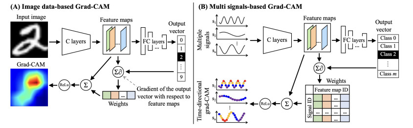
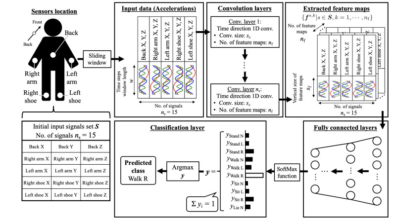
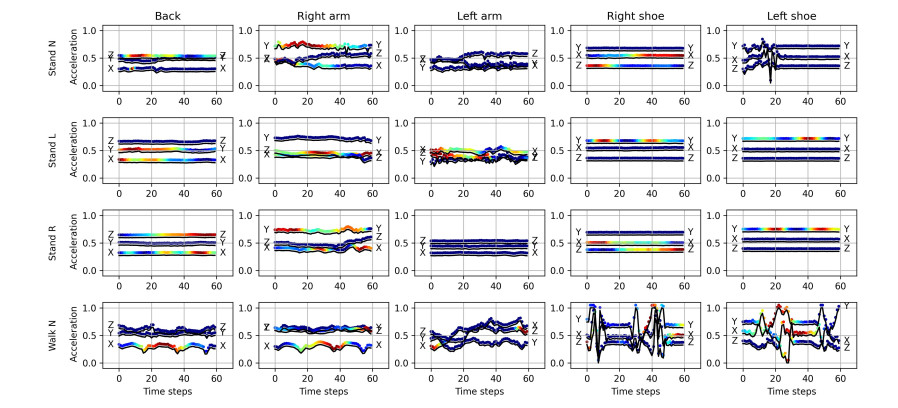
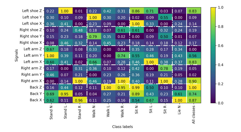
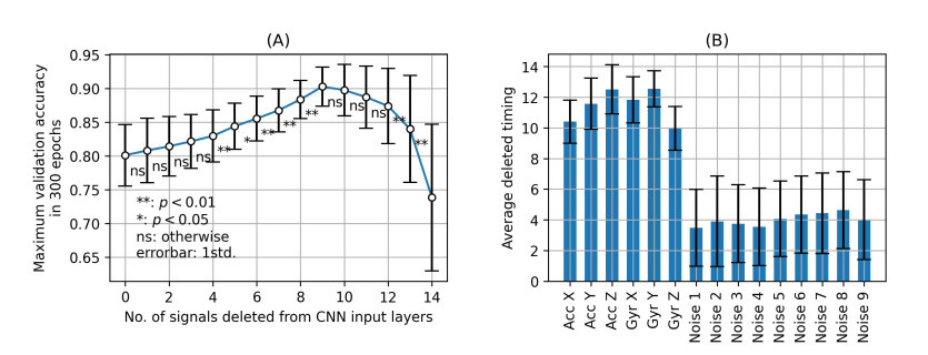
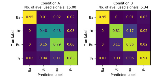
Recently, convolutional neural networks (CNNs) for classification by time domain data of multi-signals have been developed. Although some signals are important for correct classification, others are not. The calculation, memory, and data collection costs increase when data that include unimportant signals for classification are taken as the CNN input layer. Therefore, identifying and eliminating non-important signals from the input layer are important. In this study, we proposed a features gradient-based signals selection algorithm (FG-SSA), which can be used for finding and removing non-important signals for classification by utilizing features gradient obtained by the process of gradient-weighted class activation mapping (grad-CAM). When we defined $ n_ \mathrm{s} $ as the number of signals, the computational complexity of FG-SSA is the linear time $ \mathcal{O}(n_ \mathrm{s}) $ (i.e., it has a low calculation cost). We verified the effectiveness of the algorithm using the OPPORTUNITY dataset, which is an open dataset comprising of acceleration signals of human activities. In addition, we checked the average of 6.55 signals from a total of 15 signals (five triaxial sensors) that were removed by FG-SSA while maintaining high generalization scores of classification. Therefore, FG-SSA can find and remove signals that are not important for CNN-based classification. In the process of FG-SSA, the degree of influence of each signal on each class estimation is quantified. Therefore, it is possible to visually determine which signal is effective and which is not for class estimation. FG-SSA is a white-box signal selection algorithm because it can understand why the signal was selected. The existing method, Bayesian optimization, was also able to find superior signal sets, but the computational cost was approximately three times greater than that of FG-SSA. We consider FG-SSA to be a low-computational-cost algorithm.
Citation: Yuto Omae, Yusuke Sakai, Hirotaka Takahashi. Features gradient-based signals selection algorithm of linear complexity for convolutional neural networks[J]. AIMS Mathematics, 2024, 9(1): 792-817. doi: 10.3934/math.2024041
Recently, convolutional neural networks (CNNs) for classification by time domain data of multi-signals have been developed. Although some signals are important for correct classification, others are not. The calculation, memory, and data collection costs increase when data that include unimportant signals for classification are taken as the CNN input layer. Therefore, identifying and eliminating non-important signals from the input layer are important. In this study, we proposed a features gradient-based signals selection algorithm (FG-SSA), which can be used for finding and removing non-important signals for classification by utilizing features gradient obtained by the process of gradient-weighted class activation mapping (grad-CAM). When we defined $ n_ \mathrm{s} $ as the number of signals, the computational complexity of FG-SSA is the linear time $ \mathcal{O}(n_ \mathrm{s}) $ (i.e., it has a low calculation cost). We verified the effectiveness of the algorithm using the OPPORTUNITY dataset, which is an open dataset comprising of acceleration signals of human activities. In addition, we checked the average of 6.55 signals from a total of 15 signals (five triaxial sensors) that were removed by FG-SSA while maintaining high generalization scores of classification. Therefore, FG-SSA can find and remove signals that are not important for CNN-based classification. In the process of FG-SSA, the degree of influence of each signal on each class estimation is quantified. Therefore, it is possible to visually determine which signal is effective and which is not for class estimation. FG-SSA is a white-box signal selection algorithm because it can understand why the signal was selected. The existing method, Bayesian optimization, was also able to find superior signal sets, but the computational cost was approximately three times greater than that of FG-SSA. We consider FG-SSA to be a low-computational-cost algorithm.

| [1] |
N. Shahini, Z. Bahrami, S. Sheykhivand, S. Marandi, M. Danishvar, S. Danishvar, et al., Automatically identified EEG signals of movement intention based on CNN network (end-to-end), Electronics, 11 (2022), 3297. https://doi.org/10.3390/electronics11203297 doi: 10.3390/electronics11203297

|
| [2] | T. Zebin, P. J. Scully, K. B. Ozanyan, Human activity recognition with inertial sensors using a deep learning approach, Proceedings IEEE Sensors, (2017), 1–3. https://doi.org/10.1109/ICSENS.2016.7808590 |
| [3] | W. Xu, Y. Pang, Y. Yang, Y. Liu, Human activity recognition based on convolutional neural network, Proceedings of the International Conference on Pattern Recognition, (2018), 165–170. https://doi.org/10.1109/ICPR.2018.8545435 |
| [4] |
Y. Omae, M. Kobayashi, K. Sakai, T. Akiduki, A. Shionoya, H. Takahashi, Detection of swimming stroke start timing by deep learning from an inertial sensor, ICIC Express Letters Part B: Applications ICIC International, 11 (2020), 245–251. https://doi.org/10.24507/icicelb.11.03.245 doi: 10.24507/icicelb.11.03.245
|
| [5] | D. Sagga, A. Echtioui, R. Khemakhem, M. Ghorbel, Epileptic seizure detection using EEG signals based on 1D-CNN approach, Proceedings of the 20th International Conference on Sciences and Techniques of Automatic Control and Computer Engineering, (2020), 51–56. https://doi.org/10.1109/STA50679.2020.9329321 |
| [6] |
N. Dua, S. N. Singh, V. B. Semwal, Multi-input CNN-GRU based human activity recognition using wearable sensors, Computing, 103 (2021), 1461–1478. https://doi.org/10.1007/s00607-021-00928-8 doi: 10.1007/s00607-021-00928-8
|
| [7] | Y. H. Yeh, D. P. Wong, C. T. Lee, P. H. Chou, Deep learning-based real-time activity recognition with multiple inertial sensors, Proceedings of the 2022 4th International Conference on Image, Video and Signal Processing, (2022), 92–99. https://doi.org/10.1145/3531232.3531245 |
| [8] | J. P. Wolff, F. Grützmacher, A. Wellnitz, C. Haubelt, Activity recognition using head worn inertial sensors, Proceedings of the 5th International Workshop on Sensor-based Activity Recognition and Interaction, (2018), 1–7. https://doi.org/10.1145/3266157.3266218 |
| [9] |
R. R. Selvaraju, M. Cogswell, A. Das, R. Vedantam, D. Parikh, D. Batra, Grad-CAM: Visual explanations from deep networks via gradient-based localization, Int. J. Comput. Vision, 128 (2016), 336–359. https://doi.org/10.1109/ICCV.2017.74 doi: 10.1109/ICCV.2017.74
|
| [10] | B. Zhou, A. Khosla, A. Lapedriza, A. Oliva, A. Torralba, Learning deep features for discriminative localization, Proceedings of the IEEE Conference on Computer Vision and Pattern Recognition, (2016), 2921–2929. |
| [11] |
M. Kara, Z. Öztürk, S. Akpek, A. A. Turupcu, P. Su, Y. Shen, COVID-19 diagnosis from chest ct scans: A weakly supervised CNN-LSTM approach, AI, 2 (2021), 330–341. https://doi.org/10.3390/ai2030020 doi: 10.3390/ai2030020
|
| [12] | M. Kavitha, N. Yudistira, T. Kurita, Multi instance learning via deep CNN for multi-class recognition of Alzheimer's disease, 2019 IEEE 11th International Workshop on Computational Intelligence and Applications, (2019), 89–94. https://doi.org/10.1109/IWCIA47330.2019.8955006 |
| [13] |
J. G. Nam, J. Kim, K. Noh, H. Choi, D. S. Kim, S. J. Yoo, et al., Automatic prediction of left cardiac chamber enlargement from chest radiographs using convolutional neural network, Eur. Radiol., 31 (2021), 8130–8140. https://doi.org/10.1007/s00330-021-07963-1 doi: 10.1007/s00330-021-07963-1
|
| [14] |
T. Matsumoto, S. Kodera, H. Shinohara, H. Ieki, T. Yamaguchi, Y. Higashikuni, et al., Diagnosing heart failure from chest X-ray images using deep learning, Int. Heart J., 61 (2020), 781–786. https://doi.org/10.1536/ihj.19-714 doi: 10.1536/ihj.19-714
|
| [15] |
Y. Hirata, K. Kusunose, T. Tsuji, K. Fujimori, J. Kotoku, M. Sata, Deep learning for detection of elevated pulmonary artery wedge pressure using standard chest X-ray, Can. J. Cardiol., 37 (2021), 1198–1206. https://doi.org/10.1016/j.cjca.2021.02.007 doi: 10.1016/j.cjca.2021.02.007
|
| [16] |
M. Dutt, S. Redhu, M. Goodwin, C. W. Omlin, SleepXAI: An explainable deep learning approach for multi-class sleep stage identification, Appl. Intell., 53 (2023), 16830–16843. https://doi.org/10.1007/s10489-022-04357-8 doi: 10.1007/s10489-022-04357-8
|
| [17] |
S. Jonas, A. O. Rossetti, M. Oddo, S. Jenni, P. Favaro, F. Zubler, EEG-based outcome prediction after cardiac arrest with convolutional neural networks: Performance and visualization of discriminative features, Human Brain Mapp., 40 (2019), 4606–4617. https://doi.org/10.1002/hbm.24724 doi: 10.1002/hbm.24724
|
| [18] |
C. Barros, B. Roach, J. M. Ford, A. P. Pinheiro, C. A. Silva, From sound perception to automatic detection of schizophrenia: An EEG-based deep learning approach, Front. Psychiatry, 12 (2022), 813460. https://doi.org/10.3389/fpsyt.2021.813460 doi: 10.3389/fpsyt.2021.813460
|
| [19] |
Y. Yan, H. Zhou, L. Huang, X. Cheng, S. Kuang, A novel two-stage refine filtering method for EEG-based motor imagery classification, Front. Neurosci., 15 (2021), 657540. https://doi.org/10.3389/fnins.2021.657540 doi: 10.3389/fnins.2021.657540
|
| [20] |
M. Porumb, S. Stranges, A. Pescapè, L. Pecchia, Precision medicine and artificial intelligence: A pilot study on deep learning for hypoglycemic events detection based on ECG, Sci. Rep-UK., 10 (2020), 170. https://doi.org/10.1038/s41598-019-56927-5 doi: 10.1038/s41598-019-56927-5
|
| [21] |
S. Raghunath, A. E. U. Cerna, L. Jing, D. P. vanMaanen, J. Stough, D. N. Hartzel, et al., Prediction of mortality from 12-lead electrocardiogram voltage data using a deep neural network, Nat. Med., 26 (2020), 886–891. https://doi.org/10.1038/s41591-020-0870-z doi: 10.1038/s41591-020-0870-z
|
| [22] |
H. Shin, Deep convolutional neural network-based hemiplegic gait detection using an inertial sensor located freely in a pocket, Sensors, 22 (2022), 1920. https://doi.org/10.3390/s22051920 doi: 10.3390/s22051920
|
| [23] |
G. Aquino, M. G. Costa, C. F. C. Filho, Explaining one-dimensional convolutional models in human activity recognition and biometric identification tasks, Sensors, 22 (2022), 5644. https://doi.org/10.3390/s22155644 doi: 10.3390/s22155644
|
| [24] |
R. Ge, M. Zhou, Y. Luo, Q. Meng, G. Mai, D. Ma, et al, , Mctwo: A two-step feature selection algorithm based on maximal information coefficient, BMC Bioinformatics, 17 (2016), 142. https://doi.org/10.1186/s12859-016-0990-0 doi: 10.1186/s12859-016-0990-0
|
| [25] | T. Naghibi, S. Hoffmann, B. Pfister, Convex approximation of the NP-hard search problem in feature subset selection, 2013 IEEE International Conference on Acoustics, Speech and Signal Processing, (2013), 3273–3277. https://doi.org/10.1109/ICASSP.2013.6638263 |
| [26] |
D. S. Hochba, Approximation algorithms for NP-hard problems, ACM SIGACT News, 28 (1997), 40–52. https://doi.org/10.1145/261342.571216 doi: 10.1145/261342.571216
|
| [27] | C. Yun, J. Yang, Experimental comparison of feature subset selection methods, Seventh IEEE International Conference on Data Mining Workshops, (2007), 367–372. https://doi.org/10.1109/ICDMW.2007.77 |
| [28] |
W. C. Lin, Experimental study of information measure and inter-intra class distance ratios on feature selection and orderings, IEEE T. Syst. Man Cy-S, 3 (1973), 172–181. https://doi.org/10.1109/TSMC.1973.5408500 doi: 10.1109/TSMC.1973.5408500
|
| [29] |
W. Y. Loh, Classification and regression trees, Data Mining and Knowledge Discovery, 1 (2011), 14–23. https://doi.org/10.1002/widm.8 doi: 10.1002/widm.8
|
| [30] | M. R. Osborne, B. Presnell, B. A. Turlach, On the lasso and its dual, J. Comput. Graph. Stat., 9 (2000), 319–337. https://doi.org/10.1080/10618600.2000.10474883 |
| [31] |
R. J. Palma-Mendoza, D. Rodriguez, L. de Marcos, Distributed Relieff-based feature selection in spark, Knowl. Inf. Syst., 57 (2018), 1–20. https://doi.org/10.1007/s10115-017-1145-y doi: 10.1007/s10115-017-1145-y
|
| [32] |
Y. Huang, P. J. McCullagh, N. D. Black, An optimization of Relieff for classification in large datasets, Data Knowl. Eng., 68 (2009), 1348–1356. https://doi.org/10.1016/j.datak.2009.07.011 doi: 10.1016/j.datak.2009.07.011
|
| [33] |
R. Yao, J. Li, M. Hui, L. Bai, Q. Wu, Feature selection based on random forest for partial discharges characteristic set, IEEE Access, 8 (2020), 159151–159161. https://doi.org/10.1109/ACCESS.2020.3019377 doi: 10.1109/ACCESS.2020.3019377
|
| [34] |
M. Mori, R. G. Flores, Y. Suzuki, K. Nukazawa, T. Hiraoka, H. Nonaka, Prediction of Microcystis occurrences and analysis using machine learning in high-dimension, low-sample-size and imbalanced water quality data, Harmful Algae, 117 (2022), 102273. https://doi.org/10.1016/j.hal.2022.102273 doi: 10.1016/j.hal.2022.102273
|
| [35] |
Y. Omae, M. Mori, E2H distance-weighted minimum reference set for numerical and categorical mixture data and a Bayesian swap feature selection algorithm, Mach. Learn. Know. Extr., 5 (2023), 109–127. https://doi.org/10.3390/make5010007 doi: 10.3390/make5010007
|
| [36] |
R. Garriga, J. Mas, S. Abraha, J. Nolan, O. Harrison, G. Tadros, et al., Machine learning model to predict mental health crises from electronic health records, Nat. Med., 28 (2022), 1240–1248. https://doi.org/10.1038/s41591-022-01811-5 doi: 10.1038/s41591-022-01811-5
|
| [37] |
G. Chandrashekar, F. Sahin, A survey on feature selection methods, Comput. Electr. Eng., 40 (2014), 16–28. https://doi.org/10.1016/j.compeleceng.2013.11.024 doi: 10.1016/j.compeleceng.2013.11.024
|
| [38] | N. Gopika, M. Kowshalaya, Correlation based feature selection algorithm for machine learning, Proceedings of the 3rd International Conference on Communication and Electronics Systems, (2018), 692–695. https://doi.org/10.1109/CESYS.2018.8723980 |
| [39] |
L. Fu, B. Lu, B. Nie, Z. Peng, H. Liu, X. Pi, Hybrid network with attention mechanism for detection and location of myocardial infarction based on 12-lead electrocardiogram signals, Sensors, 20 (2020), 1020. https://doi.org/10.3390/s20041020 doi: 10.3390/s20041020
|
| [40] |
F. M. Rueda, R. Grzeszick, G. A. Fink, S. Feldhorst, M. T. Hompel, Convolutional neural networks for human activity recognition using body-worn sensors, Informatics, 5 (2018), 26. https://doi.org/10.3390/informatics5020026 doi: 10.3390/informatics5020026
|
| [41] |
T. Thenmozhi, R. Helen, Feature selection using extreme gradient boosting bayesian optimization to upgrade the classification performance of motor imagery signals for BCI, J. Neurosci. Meth., 366 (2022), 109425. https://doi.org/10.1016/j.jneumeth.2021.109425 doi: 10.1016/j.jneumeth.2021.109425
|
| [42] | R. Garnett, M. A. Osborne, S. J. Roberts, Bayesian optimization for sensor set selection, Proceedings of the 9th ACM/IEEE International Conference on Information Processing in Sensor Networks, (2019), 209–219. https://doi.org/10.1145/1791212.1791238 |
| [43] |
E. Kim, Interpretable and accurate convolutional neural networks for human activity recognition, IEEE T. Ind. Inform., 16 (2020), 7190–7198. https://doi.org/10.1109/TII.2020.2972628 doi: 10.1109/TII.2020.2972628
|
| [44] |
M. Jaén-Vargas, K. M. R. Leiva, F. Fernandes, S. B. Goncalves, M. T. Silva, D. S. Lopes, et al., Effects of sliding window variation in the performance of acceleration-based human activity recognition using deep learning models, PeerJ Comput. Sci., 8 (2022), e1052. https://doi.org/10.7717/peerj-cs.1052 doi: 10.7717/peerj-cs.1052
|
| [45] |
R. Chavarriaga, H. Sagha, A. Calatroni, S. T. Digumarti, G. Tröster, J. D. R. Millán, et al., The opportunity challenge: A benchmark database for on-body sensor-based activity recognition, Pattern Recogn. Lett., 34 (2013), 2033–2042. https://doi.org/10.1016/j.patrec.2012.12.014 doi: 10.1016/j.patrec.2012.12.014
|
| [46] | H. Sagha, S. T. Digumarti, J. D. R. Millán, R. Chavarriaga, A. Calatroni, D. Roggen, et al., Benchmarking classification techniques using the opportunity human activity dataset, 2011 IEEE International Conference on Systems, Man and Cybernetics, (2011), 36–40. doi: 10.1109/ICSMC.2011.6083628 |
| [47] |
A. Murad, J. Y. Pyun, Deep recurrent neural networks for human activity recognition, Sensors, 17 (2017), 2556. https://doi.org/10.3390/s17112556 doi: 10.3390/s17112556
|
| [48] | J. B. Yang, M. N. Nguyen, P. P. San, X. L. Li, S. Krishnaswamy, Deep convolutional neural networks on multichannel time series for human activity recognition, Proceedings of the Twenty-Fourth International Joint Conference on Artificial Intelligence, (2015), 3995–4001. |
| [49] |
O. Banos, J. M. Galvez, M. Damas, H. Pomares, I. Rojas, Window size impact in human activity recognition, Sensors, 14 (2014), 6474–6499. https://doi.org/10.3390/s140406474 doi: 10.3390/s140406474
|
| [50] |
T. Tanaka, I. Nambu, Y. Maruyama, Y. Wada, Sliding-window normalization to improve the performance of machine-learning models for real-time motion prediction using electromyography, Sensors, 22 (2022), 5005. https://doi.org/10.3390/s22135005 doi: 10.3390/s22135005
|
| [51] |
J. Wu, X. Y. Chen, H. Zhang, L. D. Xiong, H. Lei, S. H. Deng, Hyperparameter optimization for machine learning models based on bayesian optimization, J. Electron. Sci. Technol., 17 (2019), 26–40. https://doi.org/10.11989/JEST.1674-862X.80904120 doi: 10.11989/JEST.1674-862X.80904120
|
| [52] |
P. Doke, D. Shrivastava, C. Pan, Q. Zhou, Y. D. Zhang, Using CNN with bayesian optimization to identify cerebral micro-bleeds, Mach. Vision Appl., 31 (2020), 1–14. https://doi.org/10.1007/s00138-020-01087-0 doi: 10.1007/s00138-020-01087-0
|
| [53] | J. Bergstra, R. Bardenet, Y. Bengio, B. Kegl, Algorithms for hyper-parameter optimization, Adv. Neural Inf. Process. Syst., 24 (2011), 2546–2554. |
| [54] | T. Akiba, S. Sano, T. Yanase, T. Ohta, M. Koyama, Optuna: A next-generation hyperparameter optimization framework, Proceedings of the 25th ACM SIGKDD international conference on knowledge discovery & data mining, (2019), 2623–2631, https://optuna.readthedocs.io/en/stable/. doi: 10.1145/3292500.3330701 |
| [55] | H. Makino, E. Kita, Stochastic schemata exploiter-based AutoML, 2021 IEEE International Conference on Data Mining Workshops, (2021), 238–245. https://doi.org/10.1109/ICDMW53433.2021.00037 |
| [56] | P. Siirtola, P. Laurinen, J. Roning and H. Kinnunen, Efficient accelerometer-based swimming exercise tracking, IEEE SSCI 2011: Symposium Series on Computational Intelligence, (2011), 156–161. https://doi.org/10.1109/CIDM.2011.5949430 |
| [57] | G. Brunner, D. Melnyk, B. Sigfússon, R. Wattenhofer, Swimming style recognition and lap counting using a smartwatch and deep learning, 2019 International Symposium on Wearable Computers, (2019), 23–31. https://doi.org/10.1145/3341163.3347719 |
Figures(10) / Tables(3)

Yuto Omae, Yusuke Sakai, Hirotaka Takahashi. Features gradient-based signals selection algorithm of linear complexity for convolutional neural networks[J]. AIMS Mathematics, 2024, 9(1): 792-817. doi: 10.3934/math.2024041


 DownLoad: