Linear Rayleigh-Taylor instability for compressible viscoelastic fluids

Caifeng Liu; Caifeng Liu

doi:10.3934/math.2023761

AIMS Mathematics

2023, Volume 8, Issue 7: 14894-14918. doi: 10.3934/math.2023761

Previous Article Next Article

Research article Special Issues

Linear Rayleigh-Taylor instability for compressible viscoelastic fluids

Caifeng Liu ^,

School of Mathematics, Northwest University, Xi'an 710127, China

Received: 16 December 2022 Revised: 09 April 2023 Accepted: 13 April 2023 Published: 21 April 2023
MSC : 35R35, 76E17

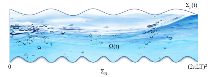
In this paper, we consider the linear Rayleigh-Taylor instability of an equilibrium state of 3D gravity-driven compressible viscoelastic fluid with the elasticity coefficient $ \kappa $ is less than a critical number $ \kappa_{c} $ in a moving horizontal periodic domain. We first construct the maximal growing mode solutions to the linearized equations by studying a family of modified variational problems, and then we prove an estimate for arbitrary solutions to the linearized equations.
- linear Rayleigh-Taylor instability,
- compressible viscoelastic fluid,
- moving domain
Citation: Caifeng Liu. Linear Rayleigh-Taylor instability for compressible viscoelastic fluids[J]. AIMS Mathematics, 2023, 8(7): 14894-14918. doi: 10.3934/math.2023761

Related Papers:

Abstract

In this paper, we consider the linear Rayleigh-Taylor instability of an equilibrium state of 3D gravity-driven compressible viscoelastic fluid with the elasticity coefficient $ \kappa $ is less than a critical number $ \kappa_{c} $ in a moving horizontal periodic domain. We first construct the maximal growing mode solutions to the linearized equations by studying a family of modified variational problems, and then we prove an estimate for arbitrary solutions to the linearized equations.

References

[1]	S. Chandrasekhar, Hydrodynamic and hydromagnetic stability, Clarendon Press, 1961.
[2]	R. Duan, F. Jiang, On the Rayleigh-Taylor instability for incompressible, inviscid magnetohydrodynamic flows, SIAM J. Appl. Math., 71 (2011), 1990–2013. https://doi.org/10.1137/110830113 doi: 10.1137/110830113
[3]	D. Ebin, Ill-posedness of the Rayleigh-Taylor and Helmholtz problems for incompressible fluids, Commun. Part. Diff. Eq., 13 (1988), 1265–1295. https://doi.org/10.1080/03605308808820576 doi: 10.1080/03605308808820576
[4]	G. L. Gui, Z. F. Zhang, Global stability of the compressible viscous surface waves in an infinite layer, 2022, arXiv: 2208.06654.
[5]	Y. Guo, I. Tice, Compressible, inviscid Rayleigh-Taylor instability, Indiana U. Math. J., 60 (2011), 677–712.
[6]	Y. Guo, I. Tice, Linear Rayleigh-Taylor instability for viscous, compressible fluids, SIAM J. Math. Anal., 42 (2010), 1688–1720. http://dx.doi.org/10.1137/090777438 doi: 10.1137/090777438
[7]	G. J. Huang, F. Jiang, W. W. Wang, On the nonlinear Rayleigh-Taylor instability of nonhomogeneous incompressible viscoelastic fluids under $L^{2}$-norm, J. Math. Anal. Appl., 455 (2017), 873–904. https://doi.org/10.1016/j.jmaa.2017.06.022 doi: 10.1016/j.jmaa.2017.06.022
[8]	H. Hwang, Y. Guo, On the dynamical Rayleigh-Taylor instability, Arch. Ration. Mech. An., 167 (2003), 235–253. https://doi.org/10.1007/s00205-003-0243-z doi: 10.1007/s00205-003-0243-z
[9]	F. Jiang, On effects of viscosity and magnetic fields on the largest growth rate of linear Rayleigh-Taylor instability, J. Math. Phys., 57 (2016), 111503. https://doi.org/10.1063/1.4966924 doi: 10.1063/1.4966924
[10]	F. Jiang, S. Jiang, On instability and stability of three-dimensional gravity flows in a bounded domain, Adv. Math., 264 (2014), 831–863. https://doi.org/10.1016/j.aim.2014.07.030 doi: 10.1016/j.aim.2014.07.030
[11]	F. Jiang, S. Jiang, On linear instability and stability of the Rayleigh-Taylor problem in magnetohydrodynamics, J. Math. Fluid Mech., 17 (2015), 639–668. https://doi.org/10.1007/s00021-015-0221-x doi: 10.1007/s00021-015-0221-x
[12]	F. Jiang, S. Jiang, On the stabilizing effect of the magnetic field in the magnetic Rayleigh-Taylor problem, SIAM J. Math. Anal., 50 (2018), 491–540. https://doi.org/10.1137/16M1069584 doi: 10.1137/16M1069584
[13]	F. Jiang, S. Jiang, G. X. Ni, Nonlinear instability for nonhomogeneous incompressible viscous fluids, Sci. China Math., 56 (2013), 665–686. https://doi.org/10.1007/s11425-013-4587-z doi: 10.1007/s11425-013-4587-z
[14]	F. Jiang, S. Jiang, Y. J. Wang, On the Rayleigh-Taylor instability for the incompressible viscous magnetohydrodynamic equations, Commun. Part. Diff. Eq., 39 (2014), 399–438. https://doi.org/10.1080/03605302.2013.863913 doi: 10.1080/03605302.2013.863913
[15]	F. Jiang, S. Jiang, G. C. Wu, On stabilizing effect of elasticity in the Rayleigh-Taylor problem of stratified viscoelastic fluids, J. Funct. Anal., 272 (2017), 3763–3824. https://doi.org/10.1016/j.jfa.2017.01.007 doi: 10.1016/j.jfa.2017.01.007
[16]	J. Jang, I. Tice, Instability theory of the Navier-Stokes-Poisson equations, Anal. PDE, 6 (2013), 1121–1181. https://doi.org/10.2140/apde.2013.6.1121 doi: 10.2140/apde.2013.6.1121
[17]	J. Jang, I. Tice, Y. J. Wang, The compressible viscous surface-internal wave problem: Nonlinear Rayleigh-Taylor instability, Arch. Ration. Mech. An., 221 (2016), 215–272. https://doi.org/10.1007/s00205-015-0960-0 doi: 10.1007/s00205-015-0960-0
[18]	H. Kull, Theory of the Rayleigh-Taylor instability, Phys. Rep., 206 (1991), 197–325. https://doi.org/10.1016/0370-1573(91)90153-D doi: 10.1016/0370-1573(91)90153-D
[19]	J. Prüss, G. Simonett, On the Rayleigh-Taylor instability for the two-phase Navier-Stokes equations, Indiana Univ. Math. J., 59 (2010), 1853–1872. https://doi.org/10.1512/iumj.2010.59.4145 doi: 10.1512/iumj.2010.59.4145
[20]	L. Rayleigh, Investigation of the character of the equilibrium of an in compressible heavy fluid of variable density, P. Lond. Math. Soc., s1-14 (1882), 170–177. https://doi.org/10.1112/plms/s1-14.1.170 doi: 10.1112/plms/s1-14.1.170
[21]	G. I. Taylor, The stability of liquid surface when accelerated in a direction perpendicular to their planes. I., Proc. Roy. Soc. London A, 201 (1950), 192–196. https://doi.org/10.1098/rspa.1950.0052 doi: 10.1098/rspa.1950.0052
[22]	W. W. Wang, Y. Y. Zhao, On the Rayleigh-Taylor instability in compressible viscoelastic fluids, J. Math. Anal. Appl., 463 (2018), 198–221. https://doi.org/10.1016/j.jmaa.2018.03.018 doi: 10.1016/j.jmaa.2018.03.018
[23]	Y. J. Wang, I. Tice, The viscous surface-internal wave problem: nonlinear Rayleigh-Taylor instability, Commun. Part. Diff. Eq., 37 (2012), 1967–2028. https://doi.org/10.1080/03605302.2012.699498 doi: 10.1080/03605302.2012.699498
[24]	Y. J. Wang, I. Tice, C. Kim, The viscous surface-internal wave problem: Global well-posedness and decay, Arch. Ration. Mech. Anal., 212 (2014), 1–92. https://doi.org/10.1007/s00205-013-0700-2 doi: 10.1007/s00205-013-0700-2
[25]	Y. Y. Zhao, W. W. Wang, On the Rayleigh-Taylor instability incompressible viscoelastic fluids under $L^{1}$-norm, J. Comput. Appl. Math., 383 (2021), 113130. https://doi.org/10.1016/j.cam.2020.113130 doi: 10.1016/j.cam.2020.113130

Reader Comments

Your name:*

Email:*
© 2023 the Author(s), licensee AIMS Press. This is an open access article distributed under the terms of the Creative Commons Attribution License (http://creativecommons.org/licenses/by/4.0)