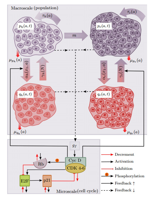
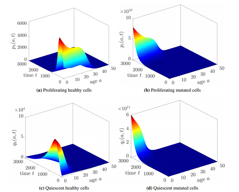
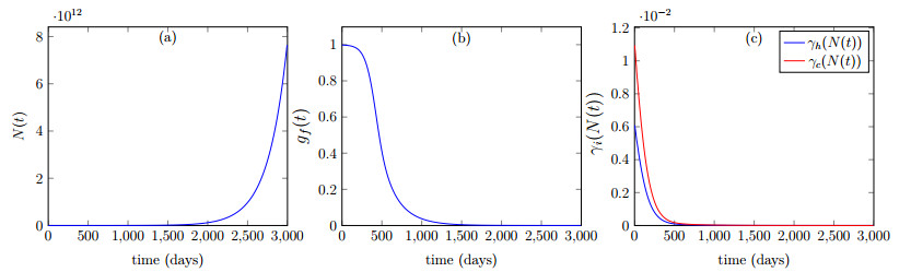
This paper presents a mathematical analysis on our proposed physiologically structured PDE model that incorporates multiscale and nonlinear features. The model accounts for both mutated and healthy populations of quiescent and proliferating cells at the macroscale, as well as the microscale dynamics of cell cycle proteins. A reversible transition between quiescent and proliferating cell populations is assumed. The growth factors generated from the total cell population of proliferating and quiescent cells influence cell cycle dynamics. As feedback from the microscale, Cyclin D/CDK 4-6 protein concentration determines the transition rates between quiescent and proliferating cell populations. Using semigroup and spectral theory, we investigate the well-posedness of the model, derive steady-state solutions, and find sufficient conditions of stability for derived solutions. In the end, we executed numerical simulations to observe the impact of the parameters on the model's nonlinear dynamics.
Citation: Iqra Batool, Naim Bajcinca. Stability analysis of a multiscale model including cell-cycle dynamics and populations of quiescent and proliferating cells[J]. AIMS Mathematics, 2023, 8(5): 12342-12372. doi: 10.3934/math.2023621
This paper presents a mathematical analysis on our proposed physiologically structured PDE model that incorporates multiscale and nonlinear features. The model accounts for both mutated and healthy populations of quiescent and proliferating cells at the macroscale, as well as the microscale dynamics of cell cycle proteins. A reversible transition between quiescent and proliferating cell populations is assumed. The growth factors generated from the total cell population of proliferating and quiescent cells influence cell cycle dynamics. As feedback from the microscale, Cyclin D/CDK 4-6 protein concentration determines the transition rates between quiescent and proliferating cell populations. Using semigroup and spectral theory, we investigate the well-posedness of the model, derive steady-state solutions, and find sufficient conditions of stability for derived solutions. In the end, we executed numerical simulations to observe the impact of the parameters on the model's nonlinear dynamics.

| [1] |
S. N. Busenberg, M. Iannelli, H. R. Thieme, Global behavior of an age-structured epidemic model, SIAM J. Math. Anal., 22 (1991), 1065–1080. https://doi.org/10.1137/0522069 doi: 10.1137/0522069

|
| [2] |
H. Inaba, Age-structured homogeneous epidemic systems with application to the MSEIR epidemic model, J. Math. Biol., 54 (2007), 101–146. https://doi.org/10.1007/s00285-006-0033-y doi: 10.1007/s00285-006-0033-y
|
| [3] |
L. Zou, S. G. Ruan, W. N. Zhang, An age-structured model for the transmission dynamics of hepatitis B, SIAM J. Appl. Math, 70 (2010), 3121–3139. https://doi.org/10.1137/090777645 doi: 10.1137/090777645
|
| [4] |
Y. Yang, S. G. Ruan, D. M. Xiao, Global stability of an age-structured virus dynamics model with Beddington-DeAngelis infection function, Math. Biosci. Eng., 12 (2015), 859–877. http://dx.doi.org/10.3934/mbe.2015.12.859 doi: 10.3934/mbe.2015.12.859
|
| [5] |
C. J. Browne, S. S. Pilyugin, Global analysis of age-structured within host virus model, Discrete Cont. Dyn. Syst. B, 18 (2013), 1999–2017. http://dx.doi.org/10.3934/dcdsb.2013.18.1999 doi: 10.3934/dcdsb.2013.18.1999
|
| [6] |
M. Gyllenberg, G. F. Webb, Age-size structure in populations with quiescence, Math. Biosci., 86 (1987), 67–95. https://doi.org/10.1016/0025-5564(87)90064-2 doi: 10.1016/0025-5564(87)90064-2
|
| [7] |
J. Dyson, R. Villella-Bressan, G. F. Webb, Asynchronous exponential growth in an age structured population of proliferating and quiescent cells, Multiscale Model. Sim., 177–178 (2002), 73–83. http://dx.doi.org/10.1016/S0025-5564(01)00097-9 doi: 10.1016/S0025-5564(01)00097-9
|
| [8] |
B. P. Ayati, G. F. Webb, A. R. A. Anderson, Computational methods and results for structured multiscale models of tumor invasion, Multiscale Model. Sim., 5 (2006), 1–20. http://dx.doi.org/10.1137/050629215 doi: 10.1137/050629215
|
| [9] |
O. Arino, E. Sanchez, G. F. Webb, Necessary and sufficient conditions for asynchronous exponential growth in age structured cell populations with quiescence, J. Math. Anal. Appl., 215 (1997), 499–513. https://doi.org/10.1006/jmaa.1997.5654 doi: 10.1006/jmaa.1997.5654
|
| [10] |
F. S. Heldt, A. R. Barr, S. Cooper, C. Bakal, B. Novak, A comprehensive model for the proliferation-quiescence decision in response to endogenous DNA damage in human cells, Proc. Nat. Acad. Sci., 115 (2018), 2532–2537. https://doi.org/10.1073/pnas.1715345115 doi: 10.1073/pnas.1715345115
|
| [11] |
D. Hanahan, R. A. Weinberg, The hallmarks of cancer, Cell, 100 (2000), 57–70. https://doi.org/10.1016/s0092-8674(00)81683-9 doi: 10.1016/s0092-8674(00)81683-9
|
| [12] |
I. Martincorena, K. M. Raine, M. Gerstung, K. J. Dawson, K. Haase, P. Van Loo, et al., Universal patterns of selection in cancer and somatic tissues, Cell, 171 (2017), 1029–1041. https://doi.org/10.1016/j.cell.2017.09.042 doi: 10.1016/j.cell.2017.09.042
|
| [13] |
B. Basse, B. C. Baguley, E. S. Marshall, W. R. Joseph, B. van Brunt, G. Wake, D. J. N. Wall, A mathematical model for analysis of the cell cycle in cell lines derived from human tumors, J. Math. Biol., 47 (2003), 295–312. https://doi.org/10.1007/s00285-003-0203-0 doi: 10.1007/s00285-003-0203-0
|
| [14] |
F. Billy, J. Clairambault, F. Delaunay, C. Feillet, N. Robert, Age-structured cell population model to study the influence of growth factors on cell cycle dynamics, Math. Biosci. Eng., 10 (2013), 1–17. https://doi.org/10.3934/mbe.2013.10.1 doi: 10.3934/mbe.2013.10.1
|
| [15] |
V. Akimenko, R. Anguelov, Steady states and outbreaks of two-phase nonlinear age-structured model of population dynamics with discrete time delay, J. Biol. Dyn., 11 (2017), 75–101. https://doi.org/10.1080/17513758.2016.1236988 doi: 10.1080/17513758.2016.1236988
|
| [16] |
E. O. Alzahrani, A. Asiri, M. M. El-Dessoky, Y. Kuang, Quiescence as an explanation of Gompertzian tumor growth revisited, Math. Biosci., 254 (2014), 76–82. https://doi.org/10.1016/j.mbs.2014.06.009 doi: 10.1016/j.mbs.2014.06.009
|
| [17] |
P. Gabriel, S. P. Garbett, V. Quaranta, D. R. Tyson, G. F. Webb, The contribution of age structure to cell population responses to targeted therapeutics, J. Theor. Biol., 311 (2012), 19–27. https://doi.org/10.1016/j.jtbi.2012.07.001 doi: 10.1016/j.jtbi.2012.07.001
|
| [18] |
Z. J. Liu, J. Chen, J. H. Pang, P. Bi, S. G. Ruan, Modeling and analysis of a nonlinear age-structured model for tumor cell populations with quiescence, J. Nonlinear Sci., 28 (2018), 1763–1791. https://doi.org/10.1007/s00332-018-9463-0 doi: 10.1007/s00332-018-9463-0
|
| [19] |
Z. J. Liu, C. F. Guo, J. Yang, H. Li, Steady states analysis of a nonlinear age-structured tumor cell population model with quiescence and bidirectional transition, Acta Appl. Math., 169 (2020), 455–474. https://doi.org/10.1007/s10440-019-00306-9 doi: 10.1007/s10440-019-00306-9
|
| [20] |
B. Britta, P. Ubezio, A generalised age- and phase-structured model of human tumour cell populations both unperturbed and exposed to a range of cancer therapies, Bull. Math. Biol., 69 (2007), 1673–1690. https://doi.org/10.1007/s11538-006-9185-6 doi: 10.1007/s11538-006-9185-6
|
| [21] | S. Cooper, On the proposal of a G0 phase and the restriction point, FASEB J., 12 (1998), 367–373. |
| [22] | A. Zetterberg, O. Larsson, Cell cycle progression and cell growth in mammalian cells: kinetic aspects of transition events, Cell Cycle Control, 24 (1995), 206–227. |
| [23] |
C. T. J. van Velthoven, T. A. Rando, Stem cell quiescence: dynamism, restraint, and cellular idling, Cell Stem Cell, 24 (2019), 213–225. https://doi.org/10.1016/j.stem.2019.01.001 doi: 10.1016/j.stem.2019.01.001
|
| [24] |
L. H. Hartwell, M. B. Kastan, Cell cycle control and cancer, Science, 266 (1994), 1821–1828. https://doi.org/10.1126/science.7997877 doi: 10.1126/science.7997877
|
| [25] |
A. Csikász-Nagy, D. Battogtokh, K. C. Chen, B. Novák, J. J. Tyson, Analysis of a generic model of eukaryotic cell-cycle regulation, Biophys. J., 90 (2006), 4361–4379. https://doi.org/10.1529/biophysj.106.081240 doi: 10.1529/biophysj.106.081240
|
| [26] |
J. E. Ferrell, T. Y. C. Tsai, Q. Yang, Modeling the cell cycle: why do certain circuits oscillate? Cell, 144 (2011), 874–885. https://doi.org/10.1016/j.cell.2011.03.006 doi: 10.1016/j.cell.2011.03.006
|
| [27] |
C. Gérard, A. Goldbeter, A skeleton model for the network of cyclin-dependent kinases driving the mammalian cell cycle, Interface Focus, 1 (2011), 24–35. https://doi.org/10.1098/rsfs.2010.0008 doi: 10.1098/rsfs.2010.0008
|
| [28] |
M. N. Obeyesekere, S. O. Zimmerman, E. S. Tecarro, G. Auchmuty, A model of cell cycle behavior dominated by kinetics of a pathway stimulated by growth factors, Bull. Math. Biol., 61 (1999), 917–934. https://doi.org/10.1006/bulm.1999.0118 doi: 10.1006/bulm.1999.0118
|
| [29] |
J. C. Sible, J. J. Tyson, Mathematical modeling as a tool for investigating cell cycle control networks, Methods, 41 (2007), 238–247. https://doi.org/10.1016/j.ymeth.2006.08.003 doi: 10.1016/j.ymeth.2006.08.003
|
| [30] |
R. Singhania, R. M. Sramkoski, J. W. Jacobberger, J. J. Tyson, A hybrid model of mammalian cell cycle regulation, PLoS Comput. Biol., 7 (2011), e1001077. https://doi.org/10.1371/journal.pcbi.1001077 doi: 10.1371/journal.pcbi.1001077
|
| [31] |
D. W. Stacey, Cyclin $\mathsf{D}$1 serves as a cell cycle regulatory switch in actively proliferating cells, Curr. Opin. Cell Biol., 15 (2003), 158–163. https://doi.org/10.1016/s0955-0674(03)00008-5 doi: 10.1016/s0955-0674(03)00008-5
|
| [32] |
R. M. Zwijsen, R. Klompmaker, E. B. Wientjens, P. M. Kristel, B. van der Burg, R. J. Michalides, Cyclin $\mathsf{D}$1 triggers autonomous growth of breast cancer cells by governing cell cycle exit, Mol. Cell. Biol., 16 (1996), 2554–2560. https://doi.org/10.1128/mcb.16.6.2554 doi: 10.1128/mcb.16.6.2554
|
| [33] |
M. Hitomi, D. W. Stacey, Cellular Ras and Cyclin $\mathsf{D}$1 are required during different cell cycle periods in cycling NIH 3T3 cells, Mol. Cell. Biol., 19 (1999), 4623–4632. https://doi.org/10.1128/mcb.19.7.4623 doi: 10.1128/mcb.19.7.4623
|
| [34] |
M. V. Blagosklonny, A. B. Pardee, The restriction point of the cell cycle, Cell Cycle, 1 (2002), 102–109. https://doi.org/10.4161/cc.1.2.108 doi: 10.4161/cc.1.2.108
|
| [35] | B. Albert, A. Johnson, J. Lewis, M. Raff, K. Roberts, P. Walter, Molecular biology of the cell, New York: Garland Science, 2002. |
| [36] |
C. P. Bagowski, J. Besser, C. R. Frey, J. E. Ferrell, The JNK cascade as a biochemical switch in mammalian cells: ultrasensitive and all-or-none responses, Curr. Biol., 13 (2003), 315–320. https://doi.org/10.1016/s0960-9822(03)00083-6 doi: 10.1016/s0960-9822(03)00083-6
|
| [37] |
C. J. Sherr, D-type cyclins, Trends Biochem. Sci., 20 (1995), 187–190. https://doi.org/10.1016/s0968-0004(00)89005-2 doi: 10.1016/s0968-0004(00)89005-2
|
| [38] |
A. D. Lander, K. K. Gokoffski, F. Y. M. Wan, Q. Nie, A. L. Calof, Cell lineages and the logic of proliferative control, PLoS Biol., 7 (2009), e1000015. https://doi.org/10.1371/journal.pbio.1000015 doi: 10.1371/journal.pbio.1000015
|
| [39] | M. B. Goldring, S. R. Goldring, Cytokines and cell growth control, Critical reviews in eukaryotic gene expression, 1 (1991), 301–326. |
| [40] |
D. Metcalf, Hematopoietic cytokines, Blood, 111 (2008), 485–491. https://doi.org/10.1182/blood-2007-03-079681 doi: 10.1182/blood-2007-03-079681
|
| [41] |
I. Batool, N. Bajcinca, Evolution of cancer stem cell lineage involving feedback regulation, PLoS ONE, 16 (2021), e0251481. https://doi.org/10.1371/journal.pone.0251481 doi: 10.1371/journal.pone.0251481
|
| [42] |
I. Batool, N. Bajcinca, Well-posedness of a coupled PDE-ODE model of stem cell lineage involving homeostatic regulation, Results Appl. Math., 9 (2021), 100135. https://doi.org/10.1016/j.rinam.2020.100135 doi: 10.1016/j.rinam.2020.100135
|
| [43] |
C. J. Sherr, J. M. Roberts, CDK inhibitors: positive and negative regulators of G1-phase progression, Genes Dev., 13 (1999), 1501–1512. https://doi.org/10.1101/gad.13.12.1501 doi: 10.1101/gad.13.12.1501
|
| [44] |
C. Gérard, A. Goldbeter, The cell cycle is a limit cycle, Math. Model. Nat. Phenom., 7 (2012), 126–166. https://doi.org/10.1051/mmnp/20127607 doi: 10.1051/mmnp/20127607
|
| [45] |
I. Batool, N. Bajcinca, A multiscale model of proliferating and quiescent cell populations coupled with cell cycle dynamics, Comput. Aided Chem. Eng., 51 (2022), 481–486. https://doi.org/10.1016/B978-0-323-95879-0.50081-3 doi: 10.1016/B978-0-323-95879-0.50081-3
|
| [46] | G. F. Webb, Theory of nonlinear age-dependent population dynamics, New York: Marcel Dekker, 1985. |
| [47] | S. M. Zheng, Nonlinear evolution equations, CRC Press, 2004. |
| [48] | T. Kato, Perturbation theory for linear operators, New York: Springer Science & Business Media, 2013. |
| [49] | H. J. A. M. Heijmans, The dynamical behaviour of the age-size-distribution of a cell population, In: The dynamics of physiologically structured populations, 1986,185–202. https://doi.org/10.1007/978-3-662-13159-6_5 |
| [50] |
C. Foley, S. Bernard, M. C. Mackey, Cost-effective G-CSF therapy strategies for cyclical neutropenia: mathematical modelling based hypotheses, J. Theor. Biol., 238 (2006), 754–763. https://doi.org/10.1016/j.jtbi.2005.06.021 doi: 10.1016/j.jtbi.2005.06.021
|
| [51] |
I. Batool, N. Bajcinca, Stability analysis of a multiscale model of cell cycle dynamics coupled with quiescent and proliferating cell populations, PloS one, 18 (2023), e0280621. https://doi.org/10.1371/journal.pone.0280621 doi: 10.1371/journal.pone.0280621
|
Figures(6) / Tables(2)

Iqra Batool, Naim Bajcinca. Stability analysis of a multiscale model including cell-cycle dynamics and populations of quiescent and proliferating cells[J]. AIMS Mathematics, 2023, 8(5): 12342-12372. doi: 10.3934/math.2023621


 DownLoad: