A mathematical approach for studying the fractal-fractional hybrid Mittag-Leffler model of malaria under some control factors

Shahram Rezapour; Sina Etemad; Joshua Kiddy K. Asamoah; Hijaz Ahmad; Kamsing Nonlaopon; Shahram Rezapour; Sina Etemad; Joshua Kiddy K. Asamoah; Hijaz Ahmad; Kamsing Nonlaopon

doi:10.3934/math.2023161

AIMS Mathematics

2023, Volume 8, Issue 2: 3120-3162. doi: 10.3934/math.2023161

Previous Article Next Article

Research article

A mathematical approach for studying the fractal-fractional hybrid Mittag-Leffler model of malaria under some control factors

1.
Department of Mathematics, Azarbaijan Shahid Madani University, Tabriz, Iran
2.
Department of Mathematics, Kyuing Hee University, 26 Kyungheedae-ro, Dongdaemun-gu, Seoul, Republic of Korea
3.
Department of Medical Research, China Medical University Hospital, China Medical University, Taichung, Taiwan
4.
Department of Mathematics, Kwame Nkrumah University of Science and Technology, Kumasi, Ghana
5.
Section of Mathematics, International Telematic University Uninettuno, Corso Vittorio Emanuele II, 39, 00186 Roma RM, Italy
6.
Department of Mathematics, Faculty of Science, Khon Kaen University, Khon Kaen 40002, Thailand

Received: 16 September 2022 Revised: 25 October 2022 Accepted: 01 November 2022 Published: 15 November 2022
MSC : 34A08, 65P99, 49J15

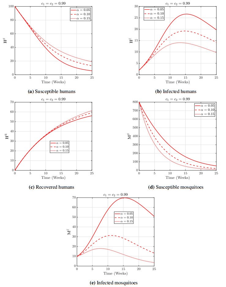
Malaria disease, which is of parasitic origin, has always been one of the challenges for human societies in areas with poor sanitation. The lack of proper distribution of drugs and lack of awareness of people in such environments cause us to see many deaths every year, especially in children under the age of five. Due to the importance of this issue, in this paper, a new five-compartmental $ (c_1, c_2) $-fractal-fractional $ \mathcal{SIR} $-$ \mathcal{SI} $-model of malaria disease for humans and mosquitoes is presented. We use the generalized Mittag-Leffler fractal-fractional derivatives to design such a mathematical model. In different ways, we study all theoretical aspects of solutions such as the existence, uniqueness and stability. A Newton polynomial that works in fractal-fractional settings is shown, which allows us to get some numerical trajectories. From the trajectories, we saw that an increase in antimalarial treatment in consideration to memory effects reduces the peak of sick individuals, and mosquito insecticide spraying minimizes the disease burden in all compartments.
- fractal-fractional hybrid operator,
- malaria,
- Newton polynomial,
- fixed point,
- stability
Citation: Shahram Rezapour, Sina Etemad, Joshua Kiddy K. Asamoah, Hijaz Ahmad, Kamsing Nonlaopon. A mathematical approach for studying the fractal-fractional hybrid Mittag-Leffler model of malaria under some control factors[J]. AIMS Mathematics, 2023, 8(2): 3120-3162. doi: 10.3934/math.2023161

Related Papers:

Abstract

Malaria disease, which is of parasitic origin, has always been one of the challenges for human societies in areas with poor sanitation. The lack of proper distribution of drugs and lack of awareness of people in such environments cause us to see many deaths every year, especially in children under the age of five. Due to the importance of this issue, in this paper, a new five-compartmental $ (c_1, c_2) $-fractal-fractional $ \mathcal{SIR} $-$ \mathcal{SI} $-model of malaria disease for humans and mosquitoes is presented. We use the generalized Mittag-Leffler fractal-fractional derivatives to design such a mathematical model. In different ways, we study all theoretical aspects of solutions such as the existence, uniqueness and stability. A Newton polynomial that works in fractal-fractional settings is shown, which allows us to get some numerical trajectories. From the trajectories, we saw that an increase in antimalarial treatment in consideration to memory effects reduces the peak of sick individuals, and mosquito insecticide spraying minimizes the disease burden in all compartments.

References

[1]	A. Prabowo, Malaria: Mencegah dan Mengatasi. (SI), Niaga Swadaya, 2004.
[2]	L. Cai, M. Martcheva, X. Z. Li, Epidemic models with age of infection, indirect transmission and incomplete treatment, Discrete Contin. Dyn. Syst. B, 18 (2013), 2239–2265. https://doi.org/10.3934/dcdsb.2013.18.2239 doi: 10.3934/dcdsb.2013.18.2239
[3]	K. W. Blayneh, J. Mohammed-Awel, Insecticide-resistant mosquitoes and malaria control, Math. Biosci., 252 (2014), 14–26. https://doi.org/10.1016/j.mbs.2014.03.007 doi: 10.1016/j.mbs.2014.03.007
[4]	H. M. Yang, A mathematical model for malaria transmission relating global warming and local socioeconomic conditions, Rev. Saude Publica, 35 (2001), 224–231. https://doi.org/10.1590/s0034-89102001000300002 doi: 10.1590/s0034-89102001000300002
[5]	C. Chiyaka, J. M. Tchuenche, W. Garira, S. Dube, A mathematical analysis of the effects of control strategies on the transmission dynamics of malaria, Appl. Math. Comput., 195 (2008), 641–662. https://doi.org/10.1016/j.amc.2007.05.016 doi: 10.1016/j.amc.2007.05.016
[6]	M. Rafikov, L. Bevilacqua, A. P. P. Wyse, Optimal control strategy of malaria vector using genetically modified mosquitoes, J. Theor. Biol., 258 (2009), 418–425. https://doi.org/10.1016/j.jtbi.2008.08.006 doi: 10.1016/j.jtbi.2008.08.006
[7]	S. Mandal, R. R. Sarkar, S. Sinha, Mathematical models of malaria–A review, Malar. J., 10 (2011), 1–19. https://doi.org/10.1186/1475-2875-10-202 doi: 10.1186/1475-2875-10-202
[8]	F. B. Agusto, N. Marcus, K. O. Okosun, Application of optimal control to the epidemiology of malaria, Electron. J. Differ. Equ., 2012 (2012), 1–22.
[9]	M. B. Abdullahi, Y. A. Hasan, F. A. Abdullah, A mathematical model of malaria and the effectiveness of drugs, Appl. Math. Sci., 7 (2013), 3079–3095. https://doi.org/10.12988/ams.2013.13270 doi: 10.12988/ams.2013.13270
[10]	R. Senthamarai, S. Balamuralitharan, A. Govindarajan, Application of homotopy analysis method in SIRS-SI model of malaria disease, Int. J. Pure Appl. Math., 113 (2017), 239–248.
[11]	P. Kumar, V. S. Erturk, The analysis of a time delay fractional COVID-19 model via Caputo type fractional derivative, Math. Methods Appl. Sci., 2022 (2022), 1–14. https://doi.org/10.1002/mma.6935 doi: 10.1002/mma.6935
[12]	A. G. Selvam, J. Alzabut, D. A. Vianny, M. Jacintha, F. B. Yousef, Modeling and stability analysis of the spread of novel coronavirus disease COVID-19, Int. J. Biomath., 14 (2021), 2150035. https://doi.org/10.1142/S1793524521500352 doi: 10.1142/S1793524521500352
[13]	S. K. Jain, S. Tyagi, N. Dhiman, J. Alzabut, Study of dynamic behaviour of psychological stress during COVID-19 in India: a mathematical approach, Res. Phys., 29 (2021), 104661. https://doi.org/10.1016/j.rinp.2021.104661 doi: 10.1016/j.rinp.2021.104661
[14]	H. Khan, R. Begum, T. Abdeljawad, M. M. Khashan, A numerical and analytical study of SE(Is)(Ih)AR epidemic fractional order COVID-19 model, Adv. Differ. Equ., 2021 (2021), 293. https://doi.org/10.1186/s13662-021-03447-0 doi: 10.1186/s13662-021-03447-0
[15]	M. Aslam, R. Murtaza, T. Abdeljawad, G. ur Rahman, A. Khan, H. Khan, et al., A fractional order HIV/AIDS epidemic model with Mittag-Leffler kernel, Adv. Differ. Equ., 2021 (2021), 107. https://doi.org/10.1186/s13662-021-03264-5 doi: 10.1186/s13662-021-03264-5
[16]	S. Rezapour, S. Etemad, H. Mohammadi, A mathematical analysis of a system of Caputo-Fabrizio fractional differential equationsfor the anthrax disease model in animals, Adv. Differ. Equ., 2020 (2020), 481. https://doi.org/10.1186/s13662-020-02937-x doi: 10.1186/s13662-020-02937-x
[17]	H. M. Alshehri, A. Khan, A fractional order Hepatitis C mathematical model with Mittag-Leffler kernel, J. Funct. Spaces, 2021 (2021), 2524027. https://doi.org/10.1155/2021/2524027 doi: 10.1155/2021/2524027
[18]	C. T. Deressa, S. Etemad, S. Rezapour, On a new four-dimensional model of memristor-based chaotic circuit in the context of nonsingular Atangana-Baleanu-Caputo operators, Adv. Differ. Equ., 2021 (2021), 444. https://doi.org/10.1186/s13662-021-03600-9 doi: 10.1186/s13662-021-03600-9
[19]	C. T. Deressa, S. Etemad, M. K. A. Kaabar, S. Rezapour, Qualitative analysis of a hyperchaotic Lorenz-Stenflo mathematical modelvia the Caputo fractional operator, J. Funct. Spaces, 2022 (2022), 4975104. https://doi.org/10.1155/2022/4975104 doi: 10.1155/2022/4975104
[20]	P. Kumar, V. S. Erturk, Environmental persistence influences infection dynamics for a butterfly pathogen via new generalised Caputo type fractional derivative, Chaos, Solitons Fract., 144 (2021), 110672. https://doi.org/10.1016/j.chaos.2021.110672 doi: 10.1016/j.chaos.2021.110672
[21]	A. Devi, A. Kumar, T. Abdeljawad, A. Khan, Stability analysis of solutions and existence theory of fractional Lagevin equation, Alex. Eng. J., 60 (2021), 3641–3647. https://doi.org/10.1016/j.aej.2021.02.011 doi: 10.1016/j.aej.2021.02.011
[22]	A. Pratap, R. Raja, R. P. Agarwal, J. Alzabut, M. Niezabitowski, E. Hincal, Further results on asymptotic and finite-time stability analysis of fractional-order time-delayed genetic regulatory networks, Neurocomputing, 475 (2022), 26–37. https://doi.org/10.1016/j.neucom.2021.11.088 doi: 10.1016/j.neucom.2021.11.088
[23]	H. Mohammadi, S. Kumar, S. Rezapour, S. Etemad, A theoretical study of the Caputo-Fabrizio fractional modeling for hearing loss due to Mumps virus with optimal control, Chaos, Solitons Fract., 144 (2021), 110668. https://doi.org/10.1016/j.chaos.2021.110668 doi: 10.1016/j.chaos.2021.110668
[24]	R. Begum, O. Tunc, H. Khan, H. Gulzar, A. Khan, A fractional order Zika virus model with Mittag-Leffler kernel, Chaos, Solitons Fract., 146 (2021), 110898. https://doi.org/10.1016/j.chaos.2021.110898 doi: 10.1016/j.chaos.2021.110898
[25]	A. Ali, Q. Iqbal, J. K. K. Asamoah, S. Islam, Mathematical modeling for the transmission potential of Zika virus with optimal control strategies, Eur. Phys. J. Plus, 137 (2022), 146. https://doi.org/10.1140/epjp/s13360-022-02368-5 doi: 10.1140/epjp/s13360-022-02368-5
[26]	P. Kumar, V. S. Erturk, H. Almusawa, Mathematical structure of mosaic disease using microbial biostimulants via Caputo and Atangana-Baleanu derivatives, Res. Phys., 24 (2021), 104186. https://doi.org/10.1016/j.rinp.2021.104186 doi: 10.1016/j.rinp.2021.104186
[27]	R. Zarin, H. Khaliq, A. Khan, D. Khan, A. Akgul, U. W. Humphries, Deterministic and fractional modeling of a computer virus propagation, Res. Phys., 33 (2022), 105130. https://doi.org/10.1016/j.rinp.2021.105130 doi: 10.1016/j.rinp.2021.105130
[28]	D. Baleanu, S. Etemad, S. Rezapour, A hybrid Caputo fractional modeling for thermostat with hybrid boundary value conditions, Bound. Value Probl., 2020 (2020), 64. https://doi.org/10.1186/s13661-020-01361-0 doi: 10.1186/s13661-020-01361-0
[29]	C. Thaiprayoon, W. Sudsutad, J. Alzabut, S. Etemad, S. Rezapour, On the qualitative analysis of the fractional boundary valueproblem describing thermostat control model via $\psi$-Hilfer fractional operator, Adv. Differ. Equ., 2021 (2021), 201. https://doi.org/10.1186/s13662-021-03359-z doi: 10.1186/s13662-021-03359-z
[30]	J. Alzabut, G. M. Selvam, R. A. El-Nabulsi, D. Vignesh, M. E. Samei, Asymptotic stability of nonlinear discrete fractionalpantograph equations with non-local initial conditions, Symmetry, 13 (2021), 473. https://doi.org/10.3390/sym13030473 doi: 10.3390/sym13030473
[31]	A. Wongcharoen, S. K. Ntouyas, J. Tariboon, Nonlocal boundary value problems for Hilfer type pantograph fractional differentialequations and inclusions, Adv. Differ. Equ., 2020 (2020), 279. https://doi.org/10.1186/s13662-020-02747-1 doi: 10.1186/s13662-020-02747-1
[32]	P. Kumar, V. S. Erturk, A. Yusuf, K. S. Nisar, S. F. Abdelwahab, A study on canine distemper virus (CDV) and rabies epidemics in the red fox population via fractional derivatives, Res. Phys., 25 (2021), 104281. https://doi.org/10.1016/j.rinp.2021.104281 doi: 10.1016/j.rinp.2021.104281
[33]	J. K. K. Asamoah, E. Okyere, E. Yankson, A. A. Opoku, A. Adom-Konadu, E. Acheampong, et al., Non-fractional and fractional mathematical analysis and simulations for Q fever, Chaos, Solitons Fract., 156 (2022), 111821. https://doi.org/10.1016/j.chaos.2022.111821 doi: 10.1016/j.chaos.2022.111821
[34]	H. Khan, C. Tunc, W. Chen, A. Khan, Existence theorems and Hyers-Ulam stability for a class of hybrid fractional differentialequations with p-Laplacial operator, J. Appl. Anal. Comput., 8 (2018), 1211–1226. https://doi.org/10.11948/2018.1211 doi: 10.11948/2018.1211
[35]	A. Omame, U. K. Nwajeri, M. Abbas, C. P. Onyenegecha, A fractional order control model for Diabetes and COVID-19 co-dynamics with Mittag-Leffler function, Alex. Eng. J., 61 (2022), 7619–7635. https://doi.org/10.1016/j.aej.2022.01.012 doi: 10.1016/j.aej.2022.01.012
[36]	D. Baleanu, S. Etemad, H. Mohammadi, S. Rezapour, A novel modeling of boundary value problems on the glucose graph, Commun. Nonlinear Sci. Numer. Simul., 100 (2021), 105844. https://doi.org/10.1016/j.cnsns.2021.105844 doi: 10.1016/j.cnsns.2021.105844
[37]	S. Rezapour, B. Tellab, C. T. Deressa, S. Etemad, K. Nonlaopon, H-U-type stability and numerical solutions for a nonlinear model of the coupled systems of Navier BVPs via the generalized differential transform method, Fractal Fract., 5 (2021), 166. https://doi.org/10.3390/fractalfract5040166 doi: 10.3390/fractalfract5040166
[38]	N. Badshah, H. Akbar, Stability analysis of fractional order SEIR model for malaria disease in Khyber Pakhtunkhwa, Demonstr. Math., 54 (2021), 326–334. https://doi.org/10.1515/dema-2021-0029 doi: 10.1515/dema-2021-0029
[39]	D. D. Pawar, W. D. Patil, D. K. Raut, Analysis of malaria dynamics using its fractional order mathematical model, J. Appl. Math. Inform., 39 (2021), 197–214. https://doi.org/10.14317/jami.2021.197 doi: 10.14317/jami.2021.197
[40]	A. ul Rehman, R. Singh, T. Abdeljawad, E. Okyere, L. Guran, Modeling, analysis and numerical solution to malaria fractional model with temporary immunity and relapse, Adv. Differ. Equ., 2021 (2021), 390. https://doi.org/10.1186/s13662-021-03532-4 doi: 10.1186/s13662-021-03532-4
[41]	X. Cui, D. Xue, T. Li, Fractional-order delayed Ross-Macdonald model for malaria transmission, Nonlinear Dyn., 107 (2022), 3155–3173. https://doi.org/10.1007/s11071-021-07114-7 doi: 10.1007/s11071-021-07114-7
[42]	M. Sinan, H. Ahmad, Z. Ahmad, J. Baili, S. Murtaza, M. A. Aiyashi, et al., Fractional mathematical modeling of malaria disease with treatment & insecticides, Res. Phys., 34 (2022), 105220. https://doi.org/10.1016/j.rinp.2022.105220 doi: 10.1016/j.rinp.2022.105220
[43]	A. Atangana, Fractal-fractional differentiation and integration: connecting fractal calculus and fractional calculus to predict complex system, Chaos, Solitons Fract., 102 (2017), 396–406. https://doi.org/10.1016/j.chaos.2017.04.027 doi: 10.1016/j.chaos.2017.04.027
[44]	J. F. Gomez-Aguilar, T. Cordova-Fraga, T. Abdeljawad, A. Khan, H. Khan, Analysis of fractal-fractional malaria transmission model, Fractals, 28 (2020), 2040041. https://doi.org/10.1142/S0218348X20400411 doi: 10.1142/S0218348X20400411
[45]	K. Shah, M. Arfan, I. Mahariq, A. Ahmadian, S. Salahshour, M. Ferrara, Fractal-fractional mathematical model addressing the situation of Corona virus in Pakistan, Res. Phys., 19 (2020), 103560. https://doi.org/10.1016/j.rinp.2020.103560 doi: 10.1016/j.rinp.2020.103560
[46]	Z. Ali, F. Rabiei, K. Shah, T. Khodadadi, Qualitative analysis of fractal-fractional order COVID-19 mathematical model with case study of Wuhan, Alex. Eng. J., 60 (2021), 477–489. https://doi.org/10.1016/j.aej.2020.09.020 doi: 10.1016/j.aej.2020.09.020
[47]	M. Alqhtani, K. M. Saad, Fractal-fractional Michaelis-Menten enzymatic reaction model via different kernels, Fractal Fract., 6 (2022), 13. https://doi.org/10.3390/fractalfract6010013 doi: 10.3390/fractalfract6010013
[48]	M. Farman, A. Akgul, K. S. Nisar, D. Ahmad, A. Ahmad, S. Kamangar, et al., Epidemiological analysis of fractional order COVID-19 model with Mittag-Leffler kernel, AIMS Math., 7 (2022), 756–783. https://doi.org/10.3934/math.2022046 doi: 10.3934/math.2022046
[49]	J. K. K. Asamoah, Fractal-fractional model and numerical scheme based on Newton polynomial for Q fever disease under Atangana-Baleanu derivative, Res. Phys., 34 (2022), 105189. https://doi.org/10.1016/j.rinp.2022.105189 doi: 10.1016/j.rinp.2022.105189
[50]	S. Etemad, I. Avci, P. Kumar, D. Baleanu, S. Rezapour, Some novel mathematical analysis on the fractal-fractional model of the AH1N1/09 virus and its generalized Caputo-type version, Chaos, Solitons Fract., 162 (2022), 112511. https://doi.org/10.1016/j.chaos.2022.112511 doi: 10.1016/j.chaos.2022.112511
[51]	H. Najafi, S. Etemad, N. Patanarapeelert, J. K. K. Asamoah, S. Rezapour, T. Sitthiwirattham, A study on dynamics of CD4$^+$ T-cells under the effect of HIV-1 infection based on a mathematical fractal-fractional model via the Adams-Bashforth scheme and Newton polynomials, Mathematics, 10 (2022), 1366. https://doi.org/10.3390/math10091366 doi: 10.3390/math10091366
[52]	D. Kumar, J. Singh, M. Al Qurashi, D. Baleanu, A new fractional SIRS-SI malaria disease model with application of vaccines, antimalarial drugs, and spraying, Adv. Differ. Equ. 2019 (2019), 278. https://doi.org/10.1186/s13662-019-2199-9 doi: 10.1186/s13662-019-2199-9
[53]	A. Granas, J. Dugundji, Fixed point theory, New York: Springer-Verlag, 2003.
[54]	A. Atangana, S. I. Araz, New numerical scheme with Newton polynomial: theory, methods, and applications, Academic Press, 2021.

Reader Comments

Your name:*

Email:*
© 2023 the Author(s), licensee AIMS Press. This is an open access article distributed under the terms of the Creative Commons Attribution License (http://creativecommons.org/licenses/by/4.0)